Robotic arm - Pick & Place project

Using Gazebo and RViz to simulate robotic arm "kuka-KR210" with 6 degree of freedom, and perform the forward and the inverse kinematics to pick an object from any shelf and place it or drop it in another place.

Gazebo, a physics based 3D simulator extensively used in the robotics world.

RViz, a 3D visualizer for sensor data analysis, and robot state visualization.

Contents :

1. Introduction
2. Installation
3. Forward Kinemtaics
4. Inverse Kinematics

1- Introduction :

The KUKA KR 210 industrial robot arm is a high payload solution for serious industrial applications. With a high payload of 210 kg and a massive reach of 2700 mm, the KR 210 KR C2 robot is ideal for a foundry setting. In fact, a foundry wrist with IP 67 protection is available with the KR 210 KR C2 instead of the standard IP 65 wrist.

Make sure you are using robo-nd VM or have Ubuntu+ROS installed locally.

2- Installation :

One time Gazebo setup step:

Check the version of gazebo installed on your system using a terminal:

$ gazebo --version

To run projects from this repository you need version 7.7.0+ If your gazebo version is not 7.7.0+, perform the update as follows:

$ sudo sh -c 'echo "deb http://packages.osrfoundation.org/gazebo/ubuntu-stable `lsb_release -cs` main" > /etc/apt/sources.list.d/gazebo-stable.list'
$ wget http://packages.osrfoundation.org/gazebo.key -O - | sudo apt-key add -
$ sudo apt-get update
$ sudo apt-get install gazebo7

Once again check if the correct version was installed:

$ gazebo --version

For the rest of this setup, catkin_ws is the name of active ROS Workspace, if your workspace name is different, change the commands accordingly

If you do not have an active ROS workspace, you can create one by:

$ mkdir -p ~/catkin_ws/src
$ cd ~/catkin_ws/
$ catkin_make

Now that you have a workspace, clone or download this repo into the src directory of your workspace:

$ cd ~/catkin_ws/src
$ git clone https://github.com/udacity/RoboND-Kinematics-Project.git

Now from a terminal window:

$ cd ~/catkin_ws
$ rosdep install --from-paths src --ignore-src --rosdistro=kinetic -y
$ cd ~/catkin_ws/src/RoboND-Kinematics-Project/kuka_arm/scripts
$ sudo chmod +x target_spawn.py
$ sudo chmod +x IK_server.py
$ sudo chmod +x safe_spawner.sh

Build the project:

$ cd ~/catkin_ws
$ catkin_make

Add following to your .bashrc file

export GAZEBO_MODEL_PATH=~/catkin_ws/src/RoboND-Kinematics-Project/kuka_arm/models

source ~/catkin_ws/devel/setup.bash

For demo mode make sure the demo flag is set to "true" in inverse_kinematics.launch file under /RoboND-Kinematics-Project/kuka_arm/launch

In addition, you can also control the spawn location of the target object in the shelf. To do this, modify the spawn_location argument in target_description.launch file under /RoboND-Kinematics-Project/kuka_arm/launch. 0-9 are valid values for spawn_location with 0 being random mode.

You can launch the project by

$ cd ~/catkin_ws/src/RoboND-Kinematics-Project/kuka_arm/scripts
$ ./safe_spawner.sh

If you are running in demo mode, this is all you need. To run your own Inverse Kinematics code change the demo flag described above to "false" and run your code (once the project has successfully loaded) by:

$ cd ~/catkin_ws/src/RoboND-Kinematics-Project/kuka_arm/scripts
$ rosrun kuka_arm IK_server.py

Once Gazebo and rviz are up and running, make sure you see following in the gazebo world:

- Robot

- Shelf

- Blue cylindrical target in one of the shelves

- Dropbox right next to the robot

If any of these items are missing, report as an issue.

Once all these items are confirmed, open rviz window, hit Next button.

To view the complete demo keep hitting Next after previous action is completed successfully.

Since debugging is enabled, you should be able to see diagnostic output on various terminals that have popped up.

The demo ends when the robot arm reaches at the top of the drop location.

There is no loopback implemented yet, so you need to close all the terminal windows in order to restart.

In case the demo fails, close all three terminal windows and rerun the script.

3- Forward Kinemtaics :

We use the forward kinematics to calculate the final coordinate position and rotation of end-effector

1. first we define our symbols

q1, q2, q3, q4, q5, q6, q7 = symbols('q1:8')
d1, d2, d3, d4, d5, d6, d7 = symbols('d1:8')
a0, a1, a2, a3, a4, a5, a6 = symbols('a0:7')
alpha0, alpha1, alpha2, alpha3, alpha4, alpha5 , alpha6 = symbols('alpha0:7')

2. using the URDF file kr210.urdf.xacro we able to know each joint position and extract an image for the robot building the DH diagram.

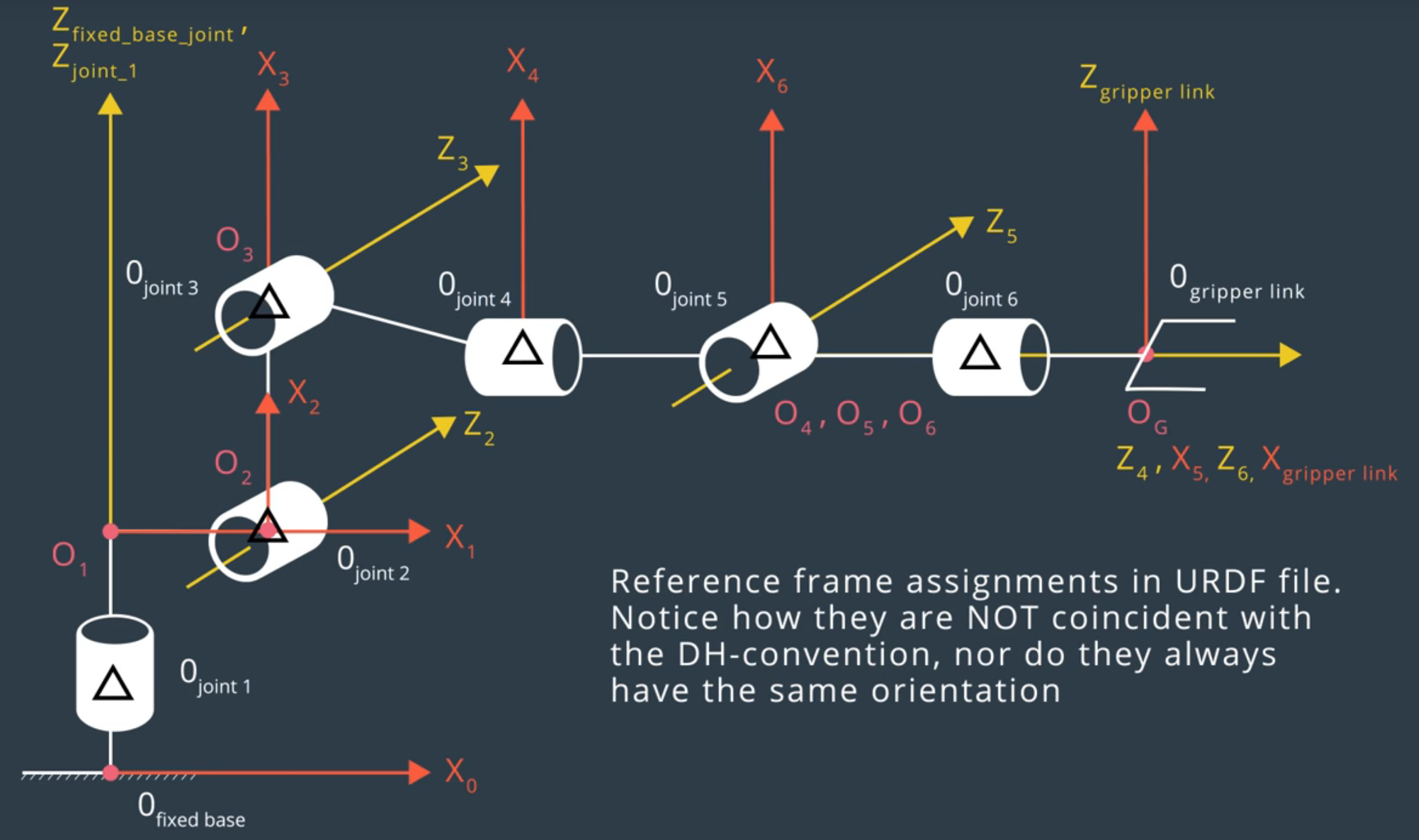
3. then we can exctract the Denavit - Hartenberg DH parameters

i	alpha	a	d	theta
1	0	0	0.75	theta_1
2	-pi/2	0.35	0	theta_2 - pi/2
3	0	1.25	0	theta_3
4	-pi/2	-0.054	1.5	theta_4
5	pi/2	0	0	theta_5
6	-pi/2	0	0	theta_6
7	0	0	0.303	theta_7

s = {alpha0:     0,  a0:     0,  d1:   0.75,
     alpha1: -pi/2,  a1:  0.35,  d2:      0, q2:  q2-pi/2,
     alpha2:     0,  a2:  1.25,  d3:      0,
     alpha3: -pi/2,  a3:-0.054,  d4:    1.5,
     alpha4:  pi/2,  a4:     0,  d5:      0,
     alpha5: -pi/2,  a5:     0,  d6:      0,
     alpha6:     0,  a6:     0,  d7:  0.303, q7:     0}

4. now we are able to define the Homogenous Transforms function to generate Homogenous Transform matrix for each joint then we can multiply the first matrix by the second by the third and so on till we get the total Homogenous Transform matrix.

to describe the relative translation and orientation of link (i-1) to link (i)

def matrix(alpha, a, d, q):
    answer = Matrix([[             cos(q),            -sin(q),            0,              a],
                     [  sin(q)*cos(alpha),  cos(q)*cos(alpha),  -sin(alpha),  -sin(alpha)*d],
                     [  sin(q)*sin(alpha),  cos(q)*sin(alpha),   cos(alpha),   cos(alpha)*d],
                     [                  0,                  0,            0,              1]])
    return answer

T0_1 = matrix(alpha=alpha0, a=a0, d=d1, q=q1)
T1_2 = matrix(alpha=alpha1, a=a1, d=d2, q=q2)
T2_3 = matrix(alpha=alpha2, a=a2, d=d3, q=q3)
T3_4 = matrix(alpha=alpha3, a=a3, d=d4, q=q4)
T4_5 = matrix(alpha=alpha4, a=a4, d=d5, q=q5)
T5_6 = matrix(alpha=alpha5, a=a5, d=d6, q=q6)
T6_G = matrix(alpha=alpha6, a=a6, d=d7, q=q7)

T0_1 = T0_1.subs(s)
T1_2 = T1_2.subs(s)
T2_3 = T2_3.subs(s)
T3_4 = T3_4.subs(s)
T4_5 = T4_5.subs(s)
T5_6 = T5_6.subs(s)
T6_G = T6_G.subs(s)

# compinsation of homogeneous transform

T0_2 = simplify(T0_1 * T1_2)
T0_3 = simplify(T0_2 * T2_3)
T0_4 = simplify(T0_3 * T3_4)
T0_5 = simplify(T0_4 * T4_5)
T0_6 = simplify(T0_5 * T5_6)
T0_G = simplify(T0_6 * T6_G)

5. we have to Compensate for rotation discrepancy between DH parameters and Gazebo

def rot_x(angle):
    R_x = Matrix([[   1,                0,               0,     0],
                [     0,       cos(angle),     -sin(angle),     0],
                [     0,       sin(angle),      cos(angle),     0],
                [     0,                0,               0,     1]])
    return R_x

def rot_y(angle):
    R_y = Matrix([[   cos(angle),                0,    sin(angle),     0],
                [             0,                1,             0,     0],
                [   -sin(angle),                0,    cos(angle),     0],
                [             0,                0,             0,     1]])
    return R_y

def rot_z(angle):
    R_z = Matrix([[      cos(angle),      -sin(angle),          0,      0],
                [       sin(angle),       cos(angle),          0,      0],
                [                0,                0,          1,      0],
                [                0,                0,          0,      1]])
    return R_z


R_corr= simplify(rot_z(np.pi) * rot_y(-np.pi/2))

T_total = simplify(T0_G * R_corr)

now we are able to get the position of the end-effector depending on the different theta angles.

4- Inverse Kinematics

1. first we have to get the end-effector position and the rotation matrix for it as following:

EE_position = Matrix([[px],[py],[pz]])
R_EE = rot_z(yaw)[0:3,0:3] * rot_y(pitch)[0:3,0:3] * rot_x(roll)[0:3,0:3] *R_corr[0:3,0:3]

WC = EE_position - 0.303*R_EE[:,2]

2. Since the last three joints in our robot are revolute and their joint axes intersect at a single point, we have a case of spherical wrist with joint_5 being the common intersection point and hence the wrist center.

This allows us to kinematically decouple the IK problem into Inverse Position and Inverse Orientation

3. first Inverse Position for the first angle theta_1, it is between x-axis and y-axis we can use tan inverse to get it

theta_1 = atan2(WC[1],WC[0])

for the second and third angles we can calculate them as following

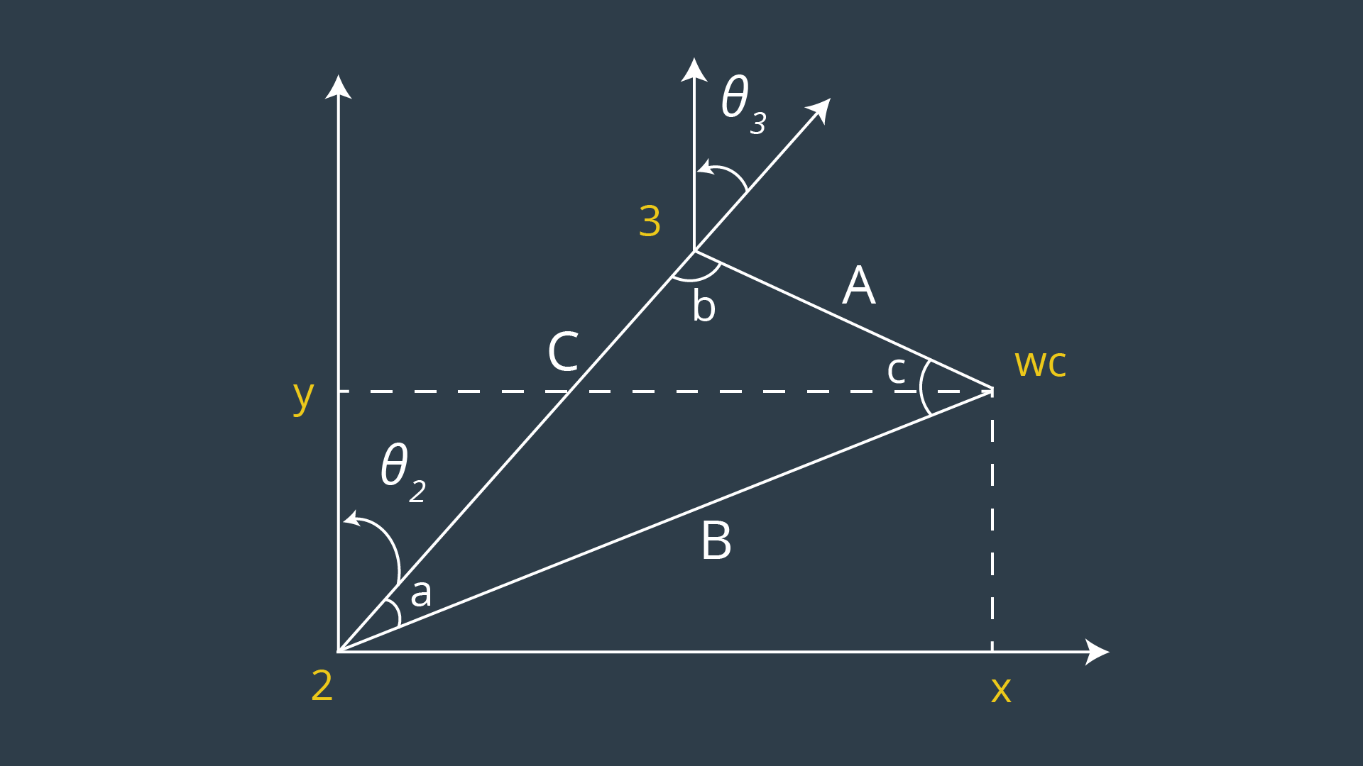
# for B
WX_new = sqrt(pow(WC[0],2) + pow(WC[1],2)) - 0.35
WZ_new = WC[2] - 0.75
branch_B = sqrt(pow(WZ_new,2) + pow(WX_new,2))

# for C and A
C = 1.25
A = 1.5

# for the other angles we need to calculate theta_2 and theta_3
angle_a = math.acos(( pow(branch_B,2) + pow(C,2) - pow(A,2) ) / ( 2 * branch_B * C ))
angle_Q = atan2(WZ_new,WX_new)
angle_b = math.acos((pow(C,2) + pow(A,2) - pow(branch_B,2)) / (2 * C * A))

#for theta_2 and theta_3
theta_2 = np.pi/2 - angle_a - angle_Q
theta_3 = np.pi/2 - angle_b - 0.03598

4. for the Inverse Orientation to calculate the last three angles

we have to calculate the rotation matrix between base link and joint 3 = R0_3 then we are able to calculate R3_6

# the rotation matrix with respect to the base link
Rrpy = R_EE

R0_3 = T0_3.evalf(subs={q1: theta_1, q2: theta_2, q3: theta_3})[0:3,0:3]

R3_6 = R0_3.inv() * Rrpy

now we can calculate the last three joints from the matrix R3_6

theta_4 = atan2(R3_6[2, 2], -R3_6[0, 2])
theta_5 = atan2(sqrt(R3_6[0, 2]*R3_6[0, 2]+R3_6[2, 2]*R3_6[2, 2]), R3_6[1, 2])
theta_6 = atan2(-R3_6[1, 1], R3_6[1, 0])