Expression Quantification

In this section we will use the aligned reads in the sorted bam format from the alignment step and count the number of reads that are mapped to annotated genomic features.

• Read counting
• Counting reads with GenomicsRanges R package
  • Counting modes
  • Workflow
• Remarks on count normalization
• Expression quantification using Tuxedo pipeline
• SCAN.UPC normalization method

Read Counting

There are three main tools that allow the quantification of reads that overlap with genomic features of interest:

1. The summarizeOverlaps() function in the GenomicRanges Bioconductor package.
2. Cuffquant/cuffnorm within the Tuxedo pipeline
3. Simple bash scripts to use htseq-count in the HTSeq Python package.

Due to time, we will focus on option 1, the summarizeOverlaps() function in the GenomicsRanges R package.

---

Counting Reads with GenomicsRanges R Package

Counting modes

Three "modes" of counting are provided to resolve reads that overlap multiple features:

• "Union"
• "IntersectionStrict"
• "IntersectionNotEmpty"

The following figure illustrates the effect of these three modes.

http://www.bioconductor.org/packages/release/bioc/vignettes/GenomicAlignments/inst/doc/summarizeOverlaps.pdf Reference

Reads mapped to a genome can be counted with summarizeOverlaps() function in the GenomicRanges R package. Reads are counted only once; there is no double-counting.

Workflow

Load the GenomicFeatures package, which contains genomic locations of desired features (transcripts, exons, genes, etc.). Extract transcript database information from GTF file.

library(GenomicFeatures)
txdb <- makeTxDbFromGFF(file="file.gtf", format="gtf")

Load GenomicRanges package, which contains the summarizeOverlaps() function to be used for read-counting.

library(GenomicRanges)

Define the features, which can be exons, transcripts, genes or any region of interest. In this case, our features of interest are genes.

eByg <- exonsBy(txdb, by="gene")

Create list of .bam files to work with.

bamdir <- "bam_sorted_indexed"
fls <- BamFileList(dir(bamdir, ".bam$", full = TRUE)) #GenomicAlignment
names(fls) <- basename(names(fls))  

Count reads mapping to genes.

genehits <- summarizeOverlaps(features=eByg, reads=aln, mode="Union")

Extract the count matrix and label the columns.

counts <- assays(genehits)$counts
counts <- as.data.frame(counts)
names(counts) <- c("g031_case", "g032_case",  "g033_case", "g034_cont", "g035_c\
ont", "g036_cont")

---

Remarks on Count Normalization

The counts quantified as above represent the raw number of reads per gene or transcript, and may be directly used as input for further studies of differential analysis between groups. However, these raw counts should not be used to report an absolute expression value; this is due to a number of factors that affect the magnitude of raw counts, the most prominent of which are

1. the total number of reads produced (library size)
2. the length of genomic features

For these reasons, raw counts must first be normalized by the above factors. This can be done using

1. RPKM: reads per kilobase per million mapped reads
2. FPKM: fragments per kilobase per million (for paired-end reads)

Note, however, this normalization does not account for other sources of bias, such as the following:

1. between-sample normalization issues
2. variations in transcript length distribution in the sample
3. coverage dependence on local sequence due to GC content
4. priming and other experimental biases
5. variability in mappability of different regions.

Important note: When the final goal is to perform differential analysis, raw counts should not be transformed into RPKM/FPKM values as this will decrease the power of statistical methods.

Expression Quantification Using Tuxedo Pipeline

The overall tuxedo workflow is depicted here:

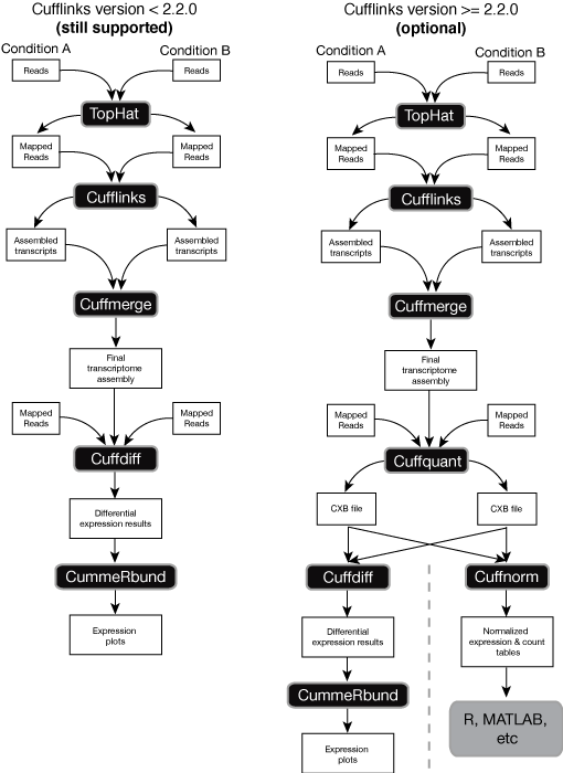
Within the the new pipeline, cuffquant and cuffnorm work together to output count tables as well as normalized expression. In the old framework, the typical work flow was to pass the Tophat alignment thorough cufflinks -> cuffmerge -> cuffdiff. This paradigm is useful when you want to predict de novo transcripts and update your *.GTF files, but you don't have to do this. Here, we directly pass the the SAM-converted output of the Tophat through cuffdiff. To compare two samples, run:

cuffdiff -o cufflinks f005_chr21_genome_annotation.gtf   sam/f031_case.sam   sam/f034_cont.sam

or for multiple sampleS:

cuffdiff -o cufflinks f005_chr21_genome_annotation.gtf   sam/f031_case.sam,sam/f032_case.sam,sam/f033_case.sam   sam/f034_cont.sam,sam/f035_cont.sam,sam/f036_cont.sam
```


## SCAN.UPC Normalization Method
-------------------------------------------------------------------------------

There is a also a new method called, called [**SCAN.UPC**](http://www.pnas.org/content/110/44/17778.full.pdf), which in addition to the factors considered in RPKM, it also corrects for the biases due to GC content. Moreover, it fits a Gaussian mixture model and transforms expression values into expression probabilities in each sample, which are more appropriate for further analysis.

UPC_RNASeq can correct for the GC content and length of each genomic region. Users
who wish to perform this correction must provide an annotation file. This tab-separated
file should contain a row for each genomic region. The first column should contain
a unique identifier that corresponds to identifiers from the read-count input file. The
second column should indicate the length of the genomic region. And the third column
should specify the number of G or C bases in the region.

```
AAB 1767 640
AAC 654 333
AAD 4644 2039
AAE 2629 1011
```

Alternatively, annotation files can be generated via the ParseMetaFromGtfFile function.
This function parses gene length and GC information from GTF files (see http:
//uswest.ensembl.org/info/website/upload/gff.html), which are used commonly
for RNA-Seq analyses.

``` R
source("http://bioconductor.org/biocLite.R")
biocLite("SCAN.UPC")
library(SCAN.UPC)
p_vec = UPC_RNASeq("ReadCounts.txt", "Annotation.txt") 
```