Convolution optimisation resources
Convolutions are probably the most used operations in both deep learning and image processing. With the rise of convolutions for sound processing, NLP and time-series, it is also critical there.
In image processing, convolutions are at the heart of blur, sharpen, emboss, edge detection and much more functions as well.
We use the deep learning terminology instead of the signal/image processing terminology.
A convolution does the following (image courtesy of Theano doc):

Input in blue, result in green, and convolution kernel or filter:

We slide the filter and a dot product between it and the input gives an element of the result.
⚠ In signal-processing this "sliding dot-product" operation is called cross-correlation. From Udacity

From the equation in the image a cross-correlation is just a flipped convolution:
Cross-correlation      Convolution
     a b c               i h g
     d e f               f e d
     g h i               c b a
For deep learning since the filter is initialised at random it doesn't matter. Cross-correlation is simpler as iteration is done in a natural way however for signal processing, convolution has the nice property of being commutative in the Fourier domain, meaning that you can precompute and fuse convolution kernels before applying them.
We will use convolution for the rest of this document.
A naive convolution of a matrix MxN with a filter k1xk2 has a computational complexity of O(MNk1k2) with data requirements of O(MN). So theoretically like GEMM (matrix multiplication also called dense, linear or affine layer) and unlike many other deep learning operations, convolutions are compute-bound and not memory-bound.
See roofline model and this presentation

Concretely that means that by using register blocking and cache blocking techniques to keep data in CPU cache we can seriously improve CPU performance similar compared to a naive implementation.
Note that for color images data requirement becomes O(MNC) and complexity O(MNCk1k2).
This is the direct implementation of the equations. From Intel paper, Anatomy of High-performance Deep Learning Convolutions on SIMD Architecture (2018-08)


Direct convolution is very memory-efficient, there is no extra allocation at all. It also works on any convolution configuration.
It's very cache-inefficient: on a popular 3x3 kernel, assuming float32, the routine will take 3 floats (CPU will load the 16 on the same cache line), then take 3 floats on next row (with 16 loads on same cache line as well) and lastly 3 floats again (with 16 loads as well). At that point, the CPU might have discarded the first row from the cache but we now need it.
All those memory issues will prevent from maximising arithmetic intensity.
Im2col is currently the most popular CPU convolution scheme. It relies on matrix multiplication (GEMM) that has been optimised for dozens of years to make the most use of CPU caches.
It does that by flattening an image to then apply GEMM. Note that an image is often "3D" in the sense that you have Height x Width x Colors (or colors are also called channels or feature maps).

It's reasonably fast, it works on any convolution configuration. Note that copying memory is O(MNC) while convolving is O(MNCk1k2) so copying penalty is dwarfed by convolution cost for big tensors (and this happens fast).
Extra MxNxC temporary memory allocation and copying is needed. This is a problem on mobile, embedded and other resource-restricted devices (for example a camera, a drone or a raspberry Pi).
- https://arxiv.org/pdf/1704.04428.pdf
-
https://arxiv.org/pdf/1709.03395.pdf
- contains on overview of GEMM-based convolutions including
- Extra memory of size O(kH*kW*C_in*H*W) ~ k² expansion
- im2col with the following copy strategies {scan, copy - self, copy - long, copy - short}
- Buffer of shape [kHkW, [HW, C_in]]
- im2row with copy strategies similar to im2col
- Buffer of shape [kHkW, [HW, C_in]]
- im2col with the following copy strategies {scan, copy - self, copy - long, copy - short}
- Extra memory of size O(kH*kW*C_out*H*W) ~ k² expansion
- kn2row
- Buffer of shape [kHkW, [C_out, HW]]
- kn2col
- Buffer of shape [kHkW, [C_out, HW]]
- kn2row
- Extra memory of size O(kH*C_in*H*W) and O(kW*C_in*H*W) ~ k expansion
- mec (memory efficient convolution)
- mec-row
- Extra memory of size O(C_out*H*W) ~ sub-k expansion
- accumulating kn2row
- Buffer of shape [[H, W], C_out]
- accumulating kn2col
- Buffer of shape [C_out, [H, W]]
- accumulating kn2row
- Extra memory of size O(k*W) ~ sub-k expansion
- hole-punching accumulating kn2row
- Buffer of shape [k,W]
- hole-punching accumulating kn2row
- Extra memory of size O(kH*kW*C_in*H*W) ~ k² expansion
- contains on overview of GEMM-based convolutions including


Convolutions are associative, a 2D kernel can sometimes be broken down into 2 1D kernels like so:
    | 1 0 -1 |   |  1 |
H = | 2 0 -2 | = |  2 | * [1 0 -1]
    | 1 0 -1 |   | -1 |
This requires k = k<sub>1</sub> = k<sub>2</sub>
This provides tremendous gain in total computational complexity as it changes from O(MNkk) to O(2*MNk).
For a 224x224 image with a 5x5 filter, this means:
2*224*224*5 = 501 760 operations instead of 224*224*5*5 = 1 254 400 operations
Assuming a 720p image (1280x720) the comparison is even more significant:
2*1280*720*5 = 9 216 000 operations instead of 1280*720*5*5 = 23 040 000 operations
For deep learning the k1k2 2D filter cannot be assumed separable but the color channel part of the filter can (remember 2D images are 3D tensors and their filters are 3D too).
So we can do a 2D spatial convolution first followed by 1D convolution on the color channel. This is called depthwise separable convolution:
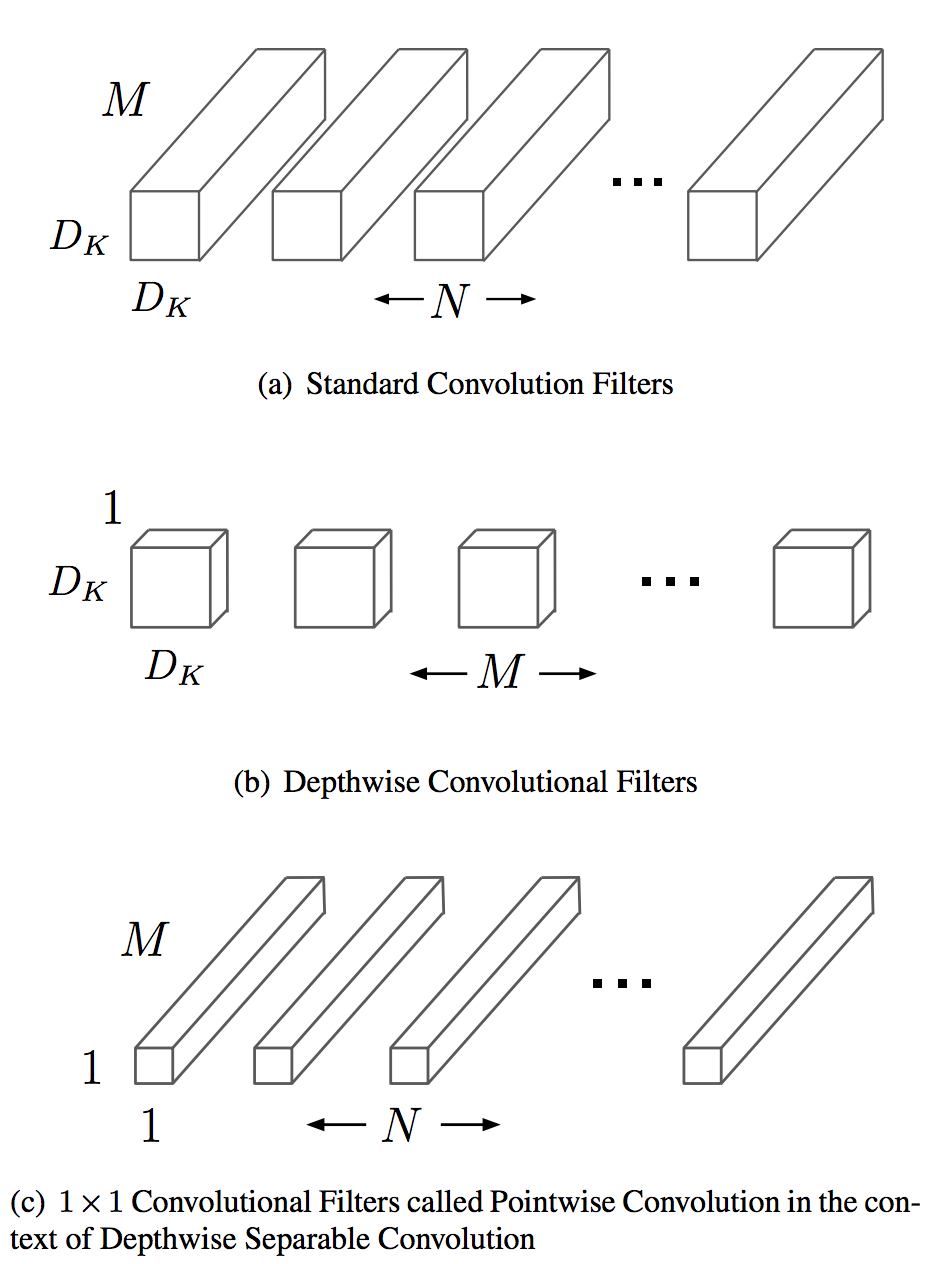
The savings are significant, for a deep-learning conv2D with the following parameters:
- Image
[C_in, H, W]for color/channel input, height, width - filter
[C_out, C_in, kH, kW]for channel output, channel input, kernel height, kernel width. (output is before input as it avoids a transposition for CHW images or NCHW batched images format)
⚠ Direct convolution is implemented as a sliding window over the preallocated output image. In the following
section we assume a stride of 1 so H ~= output_H and W ~= output_W.
A normal convolution will require kH*kW*C_in operations per sliding window so for a whole "gray" image kH*kW*C_in*H*W and now
outputting the feature channel: kH*kW*C_in*H*W*C_out
For a depthwise separable convolution we require:
- Similarly
kH*kW*C_in*H*Wfor the spatial convolution part - For the pointwise part, the sliding window requires
H*W*C_incomputations and now outputting the feature channel:H*W*C_in*C_out - The total number of operations is:
kH*kW*C_in*H*W + H*W*C_in*C_out = (H*W*C_in)*(kH*kW + C_out)
The ratio of operations between both is:
r_ops = kH*kW*C_in*H*W*C_out / ((H*W*C_in)*(kH*kW + C_out)) = kH*kW*C_out / (kH*kW + C_out)
With a similar logic, we can get the ratio of parameters in the kernel(s) between both:
r_params = kH*kW*C_in*C_out / (C_in * (kH*kW + C_out)) = kH*kW*C_out / (kH*kW + C_out)
So ratio is the same, we save as much in computation as in memory.
With real figures a 3x3 kernel with 50 output feature channels:
r = 3*3*50 / (3*3 + 50) = 7.6
Separable convolution is 7.6x more efficient than normal convolution.
Papers:
- Xception: Deep Learning with depthwise separable convolution, Chollet [1610.02357]
- MobileNets: Efficient Convolutional Neural Networks for Mobile Vision Applications, Howard et al [1704.04861]
- Depthwise Separable Convolutions for Neural Machine Translation, Kaiser et al [1706.03059]
- EffNet: an efficient structure for convolutional neural networks, Freeman et al [1801.06434]
This section gathers convolution schemes that are deep-learning specific and cannot be re-used for signal processing, as their result is not equivalent to the convolution mathematical definition. They use either the base convolution or the separable convolution as building blocks, often by having chaining convolutions over a single dimension. Those "grouped convolutions" are also sometimes called bottleneck layers.
- AlexNet, Krizhevsky et al and One weird trick to parallelize CNN [1404.5997]
- Going deeper with convolutions, Szegedy et al [1409.4842]
- Flattened Convolutional Neural Networks for Feedforward Acceleration, Jin et al [1412.5474]
- This is basically separable convolution over depth, height and width
- Deep Roots: Improving CNN efficiency with Hierarchical Filter Groups, Ioannou et al [1605.06489]
- Design of Efficient Convolutional Layers using Single Intra-channel Convolution, Topological Subdivisioning and Spatial "Bottleneck" Structure, Wang et al [1608.04337]
- Aggregated Residual Transformations for Deep Neural Networks, Xie et al [1611.05431] (ResNext)
- ShuffleNet: An extremely efficient Convolution Neural Network for Mobile Devices, Zhang et al [1707.01083]
- QuickNet: Maximizing Efficiency and Efficacy in Deep Architectures, Ghosh [1701.02291]
- Convolution with logarithmic filter groups for Efficient Shallow CNN, Tae Lee et al [1707.09855]
- Convolution speedup with CP-decomposition https://arxiv.org/pdf/1412.6553.pdf
- ChannelNet https://arxiv.org/pdf/1809.01330.pdf
- https://github.com/handong1587/handong1587.github.io/blob/master/_posts/deep_learning/2015-10-09-cnn-compression-acceleration.md
- https://github.com/gplhegde/convolution-flavors
- https://github.com/Maratyszcza/NNPACK
- Darknet
- OpenCV
- TinyDNN: https://github.com/tiny-dnn/tiny-dnn
- https://arxiv.org/pdf/1808.05567.pdf
- https://github.com/intel/mkl-dnn
- https://github.com/hfp/libxsmm
- https://github.com/ColfaxResearch/FALCON
- https://github.com/ermig1979/Simd
- uTensor (by an ARM core dev): https://github.com/utensor/utensor deep learning on 256k RAM microcontroller
- ARM NN by ARM: https://github.com/ARM-software/armnn
- NCNN by TenCent: https://github.com/Tencent/ncnn
- Paddle-mobile (ex-Mobile Deep Learning) by Baidu: https://github.com/PaddlePaddle/paddle-mobile
- https://github.com/eBay/maxDNN
- https://arxiv.org/pdf/1501.06633.pdf
- http://arxiv.org/abs/1412.7580
- https://github.com/NervanaSystems/neon/blob/master/neon/backends/winograd.py
- https://github.com/ARM-software/ComputeLibrary/tree/master/src/core/CL/kernels
- https://github.com/CNugteren/CLBlast (im2col + GEMM)
- Integral Image or Summed Area Table, a data structure to quickly compute the sum of values of rectangular subsection of an image (O(1) complexity) - Explanation - Usage in [Viola-Jones object detection framework]https://en.wikipedia.org/wiki/Viola–Jones_object_detection_framework) which allowed real-time object detection in 2001
-
Convolutional Table Ensemble https://arxiv.org/pdf/1602.04489.pdf
-
Shift: A Zero FLOP, Zero Parameter Alternative to Spatial Convolutions https://arxiv.org/abs/1711.08141
-
https://wiki.rice.edu/confluence/download/attachments/4425835/AnkushMSthesis.pdf