- Project Overview
- Data Description
- Methodology
- Results
- Python package
traffic_light_classifier - Package Usage
- Traffic light classification plays an important role in Advanced Driver Assist as well as self-driving vehicle systems which ensures timely and appropriate reaction to traffic lights in cross sections.
- In this project, a robust probabilistic approach based classifier has been implemented from scratch to classify traffic light signal's status using computer vision and machine learning techniques.
- Several data cleaning steps, features extraction and a probabilistic metric has been utilized.
- The classifier has been validated on a testing dataset with a accuracy of 99.66 %.
- All training stages and prediction stages has been throughly visualized & analyzed and thus improvised.
- The methodology utilized in this project can be generalized and applied to many other computer vision applications.
- The project presentation notebook is Notebook Traffic_Light_Classifier.
- The implemented Python package code is traffic_light_classifier.
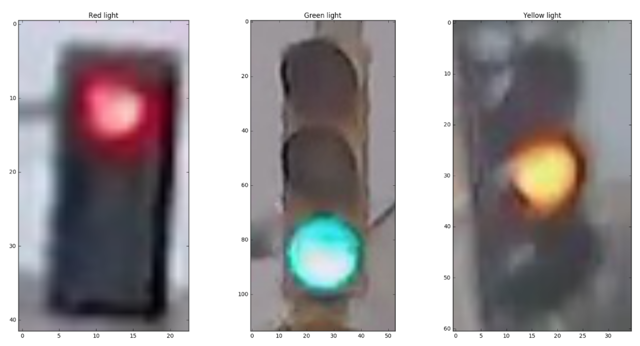
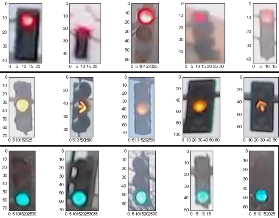
This traffic light dataset consists of 1484 number of color images in 3 categories - red, yellow, and green. As with most human-sourced data, the data is not evenly distributed among the types. There are:
- 904 red traffic light images
- 536 green traffic light images
- 44 yellow traffic light images
Note: All images come from this MIT self-driving car course and are licensed under a Creative Commons Attribution-ShareAlike 4.0 International License.
- Each image is a numpy array of shape (n_row, n_col, 3) i.e each image has a 3 channels (RGB - red, green, blue color space) where n_col and n_row is the height and the width of the image.
- Each image gives information about its colors of the pixels and their location.
- The RGB color space of the images can be converted to HSV color space channels (hue, saturation, value) i.e. the information about the hue, saturation and brightness of the pixels of the images.
The features are in the form of either rgb values or hsv values of the pixels of the image and their locations.
- Some feature extracted:
- Average hsv image for red images, yellow images & green images.
- 1D range of high saturation along width and along height for each image.
- 1D range of high brightness along width and along height for each image..
- 2D Region of high saturation for each image.
- 2D Region of high brightness for each image.
- Location of light for each image.
- Extraction of average red light hues, average yellow light hues, average green light hues from each image.
- Average s (saturation) of light located.
- Average v (bright) of light located.
- etc.
- Get average image for red, yellow and green training images.
- Get region of high saturation in average red, yellow & green images to narrow down the search window for individual images to look for the red, yellow, and green lights.
- Crop all training images at their respective color's average image's high saturation region.
- Locate lights in all images by using high saturation and high brightness regions.
- Crop images at their respective light's position
- Get average image of red light, yellow light & average green light to see the distribution of hue, saturation and brightness in red lights, yeellow light, and green lights.
- Get distribtution of hues, saturations and brightnesses of red lights, average yellow lights & green lights.
- Optimize classifier's metric's parameters for red, yellow and green lights.
- Predict & get accuracy of training dataset for classifier's optimized parameters.
For a single image, the classifier extracts the following hues from the 3 regions:
- Model's red hues from the light located in model's red light region.
- Model's yellow hues from the light located in model's yellow light region.
- Model's green hues from the light located in model's green light region.
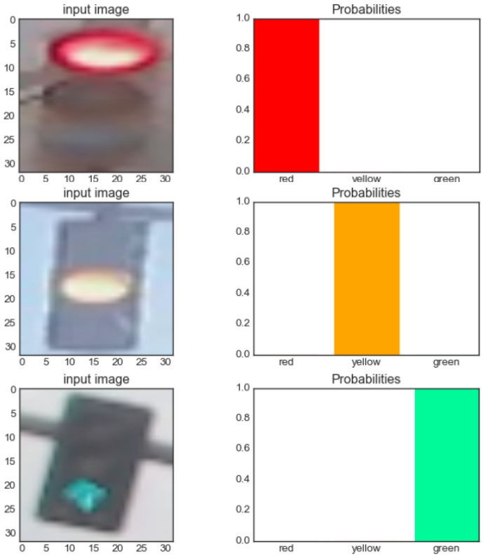
This classifier classifies an input image either red, yellow or green based on probabilities.
For a single input image, 3 lights will be located in the 3 regions (i.e. red, yellow and green light regions). Then the classifier calculates 3 probabilities:
- Probability of image being red
- Probability of image being yellow
- Probability of image being green
And propobilities are calculated by,
-
$Probability\ of\ image\ being\ red = \dfrac {strength_{red}} {strength_{red} + strength_{yellow} + strength_{green}}$ -
$Probability\ of\ image\ being\ yellow = \dfrac {strength_{yellow}} {strength_{red} + strength_{yellow} + strength_{green}}$ -
$Probability\ of\ image\ being\ green = \dfrac {strength_{green}} {strength_{red} + strength_{yellow} + strength_{green}}$ where,
$strength_{red} = \mu_{saturation_{red}}^a \times \mu_{brightness_{red}}^b$ $strength_{yellow} = \mu_{saturation_{yellow}}^a \times \mu_{brightness_{yellow}}^b$ $strength_{green} = \mu_{saturation_{green}}^a \times \mu_{brightness_{green}}^b$
and,
-
$\mu_{saturation_{red}}$ : mean saturation of the light located in model's red light region -
$\mu_{brightness_{red}}$ : mean brightness of the light located in model's red light region -
$\mu_{saturation_{yellow}}$ : mean saturation of the light located in model's yellow light region -
$\mu_{brightness_{yellow}}$ : mean brightness of the light located in model's yellow light region -
$\mu_{saturation_{green}}$ : mean saturation of the light located in model's green light region -
$\mu_{brightness_{green}}$ : mean brightness of the light located in model's green light region -
$a$ &$b$ : model's parameters
Detailed analysis and visualization of each stage has been given in Notebook Traffic_Light_Classifier.
- A custom made Python package
traffic_light_classifierhas been implemented for this project. - All training stages and prediction stages has been throughly visualized & analyzed and thus improvised.
- The classifier has been validated on a testing dataset with a accuracy of 99.66 %.
- The project results and package usage have been clearly demonstrated in the Notebook Traffic_Light_Classifier.

- This project utilizes a custom-made package
traffic_light_classifierwhich contains a classifier, plotting & feature extraction functionalities, and datasets for the project. - Libraries used:
OpenCV-Python,scipy,matplotlib,numpy. - This library offers tools which enables to analyze and visualize the entire training and prediction process stages.
# Install package from PyPI >>
!pip install traffic_light_classifier
# or
# Install package from GitHub >>
!pip install git+https://github.com/ShashankKumbhare/traffic-light-classifier.git#egg=traffic-light-classifier# Import package `traffic_light_classifier` >>
import traffic_light_classifier as tlc# Create an instance of class Model provided in the package
model = tlc.Model()# Call `compile` method of model object to train the model
# Note: Use parameter `show_analysis = True` to see the detailed process of the training/compiling stages.
model.compile()
model.compile(show_analysis = True)# Get a random red image from the test dataset provided in the package
import random
image_red = random.choice( tlc.datasets.train.images_std.red )
tlc.plots.plot_images(image_red)
# Note: Use parameter `show_probabilities = True` to see the classification probabilities.
# Use parameter `show_analysis = True` to see the detailed process of the prediction stages.
label_predicted = model.predict( image_red )
label_predicted = model.predict( image_red, show_probabilities = True )
label_predicted = model.predict( image_red, show_analysis = True )
# For yellow and green test images
image_yellow = random.choice( tlc.datasets.train.images_std.yellow )
image_green = random.choice( tlc.datasets.train.images_std.green )
label_predicted = model.predict( image_yellow, show_analysis = True )
label_predicted = model.predict( image_green, show_analysis = True )# Use `predict_dataset()` method to predict an entire dataset >>
images_std = tlc.datasets.test.images_std.all
labels_std = tlc.datasets.test.labels_std # optional
accuracy = model.predict_dataset(images_std, labels_std)
print(accuracy)An ardent user might want to see what is happening in the compiling/training process. He might also want to revisit or play with them.
# After compilation/training, all the compilation stages are stored in `model.compilation` attribute >>
# To access them:

# Compilation-Stage 1: Average image for red, yellow and green training images
image1 = model.compilation.stg1_image_avg.red
image2 = model.compilation.stg1_image_avg.yellow
image3 = model.compilation.stg1_image_avg.green
tlc.plots.plot_images([image1, image2, image3])
tlc.plots.plot_channels(image1, "hsv")
tlc.plots.plot_channels(image2, "hsv")
tlc.plots.plot_channels(image3, "hsv")

# Compilation-Stage 2a: Region of high saturation in average red, yellow & green images
print(model.compilation.stg2a_region_high_s.red)
print(model.compilation.stg2a_region_high_s.yellow)
print(model.compilation.stg2a_region_high_s.green)

# Compilation-Stage 2b: Masked average images at their respective high saturation region
image1 = model.compilation.stg2b_image_avg_masked_region_high_s.red
image2 = model.compilation.stg2b_image_avg_masked_region_high_s.yellow
image3 = model.compilation.stg2b_image_avg_masked_region_high_s.green
tlc.plots.plot_images([image1, image2, image3])
tlc.plots.plot_channels(image1, "hsv")
tlc.plots.plot_channels(image2, "hsv")
tlc.plots.plot_channels(image3, "hsv")

# Compilation-Stage 3: Cropped average images at high saturation region
images1 = model.compilation.stg3_dataset_images_cropped_high_s_region.red[0:10]
images2 = model.compilation.stg3_dataset_images_cropped_high_s_region.yellow[0:10]
images3 = model.compilation.stg3_dataset_images_cropped_high_s_region.green[0:10]
tlc.plots.plot_images(images1)
tlc.plots.plot_images(images2)
tlc.plots.plot_images(images3)

# Compilation-Stage 4: Locations of lights in all training images
print(model.compilation.stg4_locations_light.red[0:5])
print(model.compilation.stg4_locations_light.yellow[0:5])
print(model.compilation.stg4_locations_light.green[0:5])

# Compilation-Stage 5: Cropped images at their respective light's position
images1 = model.compilation.stg5_dataset_images_light.red[0:10]
images2 = model.compilation.stg5_dataset_images_light.yellow[0:10]
images3 = model.compilation.stg5_dataset_images_light.green[0:10]
tlc.plots.plot_images(images1)
tlc.plots.plot_images(images2)
tlc.plots.plot_images(images3)

# Compilation-Stage 6: Average image of red lights, yellow lights & green lights
image1 = model.compilation.stg6_image_light_avg.red
image2 = model.compilation.stg6_image_light_avg.yellow
image3 = model.compilation.stg6_image_light_avg.green
tlc.plots.plot_images([image1, image2, image3])
tlc.plots.plot_channels(image1, "hsv")
tlc.plots.plot_channels(image2, "hsv")
tlc.plots.plot_channels(image3, "hsv")

# Compilation-Stage 7: Hues, saturations and brightnesses of average red light, average yellow light & average green light
print(model.compilation.stg7a_hue_avg_light.red.mu)
print(model.compilation.stg7a_hue_avg_light.red.sigma)
print(model.compilation.stg7a_hue_avg_light.red.dist)

print(model.compilation.stg7b_sat_avg_light.red.mu)
print(model.compilation.stg7b_sat_avg_light.red.sigma)
print(model.compilation.stg7b_sat_avg_light.red.dist)

print(model.compilation.stg7c_brt_avg_light.red.mu)
print(model.compilation.stg7c_brt_avg_light.red.sigma)
print(model.compilation.stg7c_brt_avg_light.red.dist)

# Compilation-Stage 8: Optimized parameters  a & b for maximum accuracy
print(model.compilation.stg8_params_optimised)

# Compilation-Stage 9: Prediction analysis & accuracy of training dataset for classifier's optimized parameters
print( dir(model.compilation.stg9a_dataset_train_analysis.green[0]) )
print( dir(model.compilation.stg9a_dataset_train_analysis.green[0]) )
print( dir(model.compilation.stg9b_misclassified.green[0]) )
print( f"Accuracy red     = {model.compilation.stg9c_accuracy_train.red}" )
print( f"Accuracy yellow  = {model.compilation.stg9c_accuracy_train.yellow}" )
print( f"Accuracy green   = {model.compilation.stg9c_accuracy_train.yellow}" )
print( f"Accuracy overall = {model.compilation.stg9c_accuracy_train.all}" )An ardent user might want to see what is happening behind the prediction process. Analyzing misclassified images might give user the understanding of the flaws of the classifier model and help improve the algorithm.
import random
image_red = random.choice( tlc.datasets.train.images_std.red )
tlc.plots.plot_images(image_red)
label_predicted = model.predict( image_red )
# After prediction, all the compilation stages are stored in `model.prediction` attribute >>
# To access them:
# Compilation-Stage 1: Croped image at model's optimal high saturation region for red, yellow, green light's position
image1 = model.prediction.stg1_image_high_s_region.red
image2 = model.prediction.stg1_image_high_s_region.yellow
image3 = model.prediction.stg1_image_high_s_region.green
tlc.plots.plot_images([image1, image2, image3])
tlc.plots.plot_channels(image1, "hsv")
tlc.plots.plot_channels(image2, "hsv")
tlc.plots.plot_channels(image3, "hsv")

# Compilation-Stage 2: Located lights in model's optimal regions of red, yellow, green lights
model.prediction.stg2_locations_light.red
print(model.prediction.stg2_locations_light.red)
print(model.prediction.stg2_locations_light.yellow)
print(model.prediction.stg2_locations_light.green)

# Compilation-Stage 3: Cropped lights
image1 = model.prediction.stg3_image_light.red
image2 = model.prediction.stg3_image_light.yellow
image3 = model.prediction.stg3_image_light.green
tlc.plots.plot_images([image1, image2, image3])
tlc.plots.plot_channels(image1, "hsv")
tlc.plots.plot_channels(image2, "hsv")
tlc.plots.plot_channels(image3, "hsv")

# Compilation-Stage 4: Extracted model's red, yellow, green light's colors from the respective cropped parts of the input image
image1 = model.prediction.stg4_image_colors_extracted.red
image2 = model.prediction.stg4_image_colors_extracted.yellow
image3 = model.prediction.stg4_image_colors_extracted.green
tlc.plots.plot_channels(image1, "hsv")
tlc.plots.plot_channels(image2, "hsv")
tlc.plots.plot_channels(image3, "hsv")

# Compilation-Stage 5: Distribution of hues extracted from the model's red, yellow & green light region
print(model.prediction.stg5a_hue_input_light.red.mu)
print(model.prediction.stg5a_hue_input_light.red.sigma)
print(model.prediction.stg5a_hue_input_light.red.dist)

print(model.prediction.stg5a_hue_input_light.yellow.mu)
print(model.prediction.stg5a_hue_input_light.yellow.sigma)
print(model.prediction.stg5a_hue_input_light.yellow.dist)

print(model.prediction.stg5a_hue_input_light.green.mu)
print(model.prediction.stg5a_hue_input_light.green.sigma)
print(model.prediction.stg5a_hue_input_light.green.dist)
    # Similarly for saturation and brightness

# Compilation-Stage 6: Probabilities of image being red, yellow and green
print( model.prediction.stg6_probabilities.image_being_red )
print( model.prediction.stg6_probabilities.image_being_yellow )
print( model.prediction.stg6_probabilities.image_being_green )

# Compilation-Stage 7: Predicted label
print( model.prediction.stg7_label_predicted )
print( model.prediction.stg7_label_predicted_str )
The package usage have been clearly demonstrated in the Notebook Traffic_Light_Classifier.