SHPB Analysis Tool

This Python script analyses Split Hopkinson Pressure Bar (SHPB) experimental data to calculate stress-strain curves and other relevant parameters. Follow the instructions below to use the script with your experimental data.

Instructions

1. Install Dependencies: Make sure you have Python installed on your system. You can install the required Python packages by running the following command:

   pip install -r requirements.txt
   

2. Prepare Experimental Data:

   • Ensure that your experimental data is stored in a CSV or Excel file.
   • The file should contain columns for "Time", "Incident", "Reflected", and "Transmitted" voltages.
   • Voltage values should be in volts (V).
   • Specify the file name in the Python script (analysis.py) using the filename variable. For example:

   filename = "path/to/your/data_file.csv"

3. Customize Input Parameters:

   • Open the Python script (analysis.py) in a text editor.
   • Update the input parameters according to your experiment setup. Parameters such as Young's modulus, density, initial length, and cross-sectional areas should be adjusted based on your experimental conditions.

4. Run the Script:

   • Run the script using the following command:

   python analysis.py
   

5. View Plots and Analyze Results:

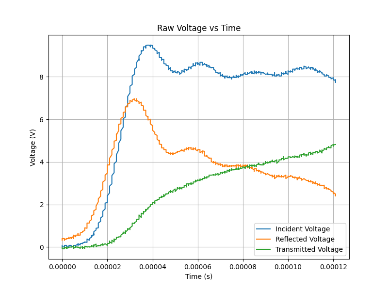
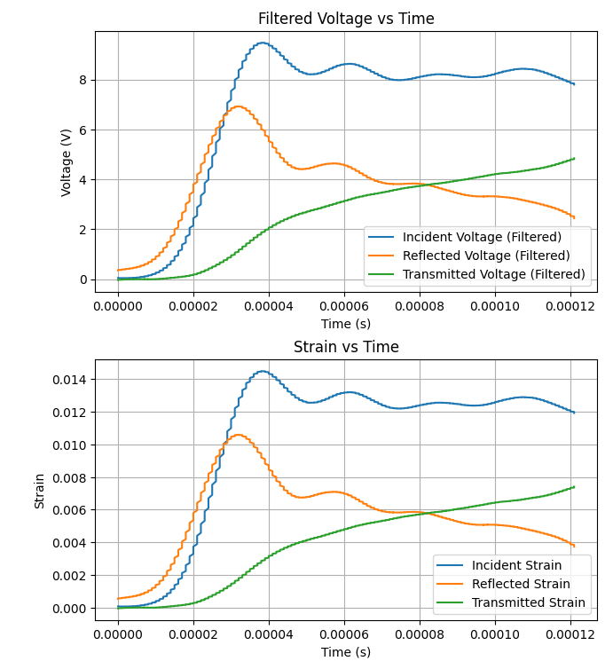
   • After running the script, view the generated plots to analyze the results.
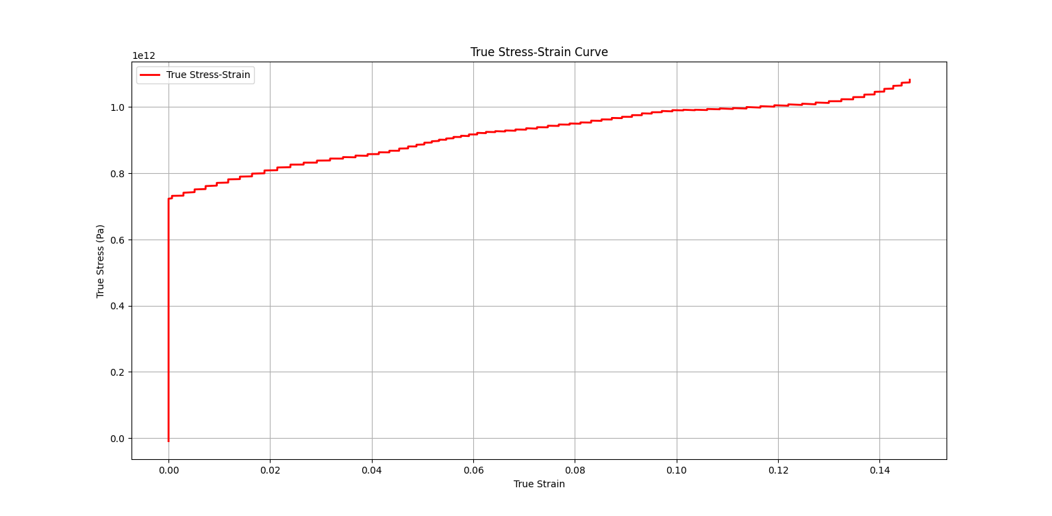
   • The script will generate plots for filtered voltage data, strain data, stress-strain curve, and true stress-strain curve.

Example Usage

Here's an example of how to use the script with your experimental data:

1. Ensure that Python and the required dependencies are installed on your system.
2. Prepare your experimental data in a CSV or Excel file format.
3. Customize the input parameters in the analysis.py script based on your experiment setup.
4. Specify the file name of your experimental data in the script.
5. Run the script using python analysis.py.
6. Analyze the generated plots to interpret the results of your SHPB experiment.

Explanation for Stress-Strain Calculation in SHPB Experiment

In the Split Hopkinson Pressure Bar (SHPB) experiment, the characteristic relations associated with one-dimensional elastic wave propagation in the bar provide the basis for calculating stress and strain in the specimen.

1. Particle Velocity at Specimen/Input-Bar and Specimen/Output-Bar Interface:

   • The particle velocity $v_1(t)$ at the specimen/input-bar interface is given by: $v_1(t) = c_b(\varepsilon_I - \varepsilon_R)$
   • Here, $c_b = \sqrt{\frac{E_b}{\rho_b}}$ represents the bar wave speed, with $E_b$ denoting the Young's modulus and $\rho_b$ the density of the bar material.
   • The particle velocity $v_2(t)$ at the specimen/output-bar interface is given by: $v_2(t) = c_b \varepsilon_T$

2. Mean Axial Strain Rate in the Specimen:

   • The mean axial strain rate $\dot{e}_s$ in the specimen is calculated as: $\dot{e}_s = \frac{c_b}{l_0} (\varepsilon_I - \varepsilon_R - \varepsilon_T) = \frac{v_1 - v_2}{l_0}$
   • Here, $l_0$ represents the initial specimen length.

3. Calculation of Bar Stresses and Normal Forces:

   • The stresses and normal forces at the specimen/bar interfaces are computed as follows:
     • $P_1 = E_b (\varepsilon_I + \varepsilon_R) A_b$ at the specimen/input-bar interface.
     • $P_2 = E_b \varepsilon_T A_b$ at the specimen/output-bar interface.
   • Here, $A_b$ denotes the cross-sectional area of the bars.

4. Mean Axial Stress in the Specimen:

   • The mean axial stress $\bar{S}_s(t)$ in the specimen is given by: $\bar{S}_s(t) = \frac{(P_1 + P_2)}{2} \left( \frac{1}{A_s} \right)$
   • Here, $A_s$ represents the initial cross-sectional area of the specimen.

5. Stress-Strain Relationship:

   • Assuming stress equilibrium, uniaxial stress conditions in the specimen, and one-dimensional elastic stress wave propagation without dispersion in the bars, the nominal strain rate $\dot{e}_s$, nominal strain $e_s$, and nominal stress $S_s$ in the specimen are estimated using:
     • $\dot{e}_s(t) = \frac{2c_b}{l_0} \varepsilon_R(t)$
     • $e_s(t) = \int_0^t \dot{e}_s(\tau) d\tau$
     • $S_s(t) = \frac{E_b A_b}{A_s} \varepsilon_T(t)$

6. True Stress-Strain:

   • True strain $\varepsilon_s(t)$ in the specimen is given by:

     • $\varepsilon_s(t) = -\ln(1 - e_s(t))$
       Here, $e_s(t)$ represents the engineering strain in the specimen.

   • The true strain rate $\dot{\varepsilon}_s(t)$ in the specimen is calculated as:

     • $\dot{\varepsilon}_s(t) = \frac{\dot{e}_s(t)}{1 - e_s(t)}$

   • The true stress $\sigma_s(t)$ in the specimen is obtained as:

     • $\sigma_s(t) = S_s(t) \cdot (1 - e_s(t))$
       Here, $S_s(t)$ represents the nominal stress in the specimen.

SHPB Cropping Tool

1. Data Preparation:

   • Prepare your SHPB data in CSV format. Each CSV file should contain three columns: 'Time' and the respective voltage data (e.g., 'Incident' and 'Transmitted').

2. Launching the Tool:

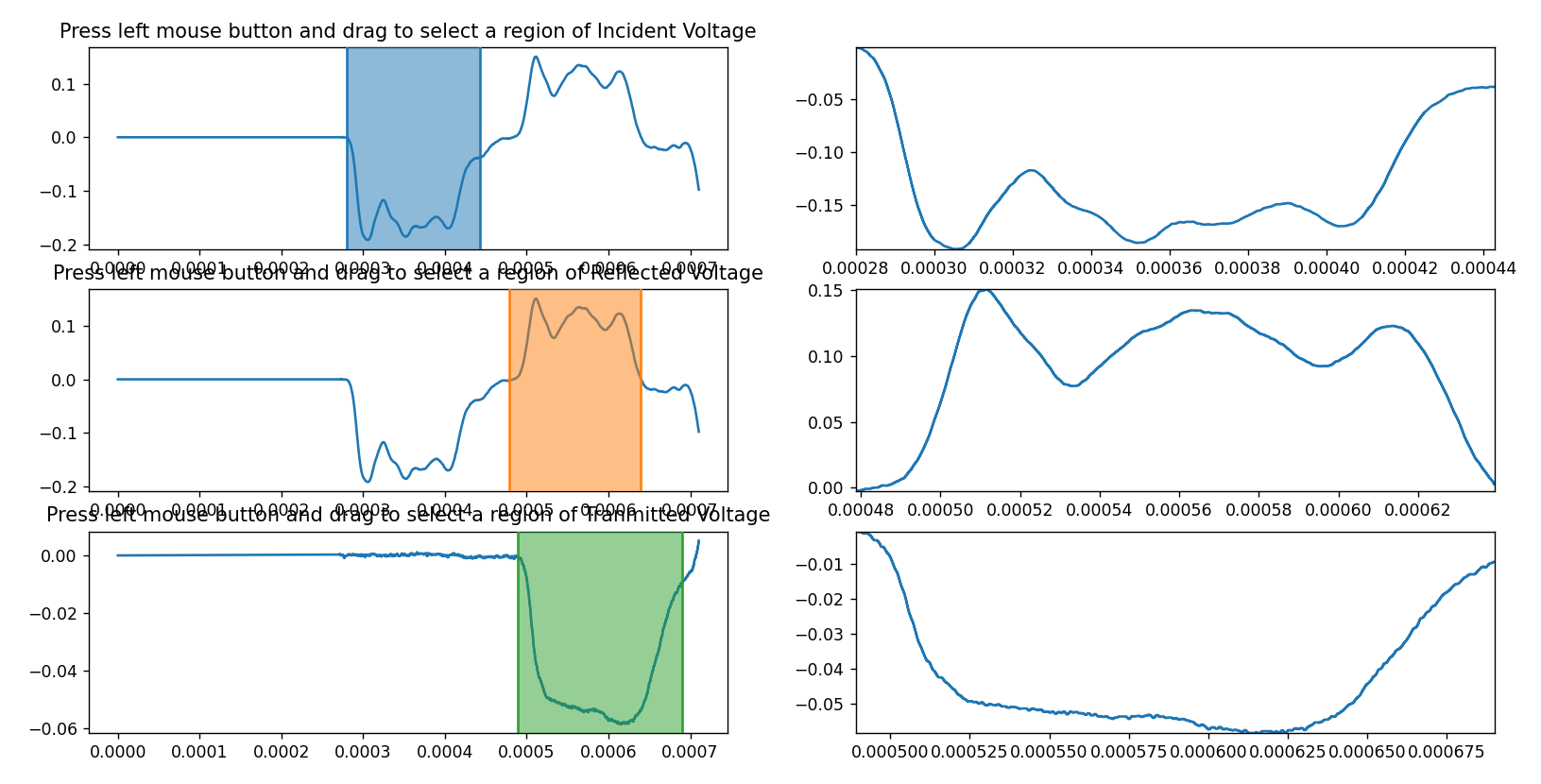
   • Run the Python script crop.py.
   • The tool will display a graphical interface with multiple subplots.

3. Selecting Regions:

   • For Incident Voltage: Click and drag on the subplot (labelled 'Incident Voltage') to select a region of interest.
   • For Reflected Voltage: Click and drag on the subplot (labelled 'Reflected Voltage') to select a region of interest.
   • For Transmitted Voltage: Click and drag on the subplot (labelled 'Transmitted Voltage') to select a region of interest.

4. Saving Selected Data:

   • The selected regions will be displayed on their respective subplots.
   • The selected data will be saved automatically to CSV files in the same directory as the script.
     • Selected Incident Voltage data will be saved to selected_incident.csv.
     • Selected Reflected Voltage data will be saved to selected_reflected.csv.
     • Selected Transmitted Voltage data will be saved to selected_transmitted.csv.

Reference

The theory and equations used in this project are based on the following sources:

• Ramesh, K.T. (2008). High Rates and Impact Experiments. In: Sharpe, W. (eds) Springer Handbook of Experimental Solid Mechanics. Springer Handbooks. Springer, Boston, MA. DOI: 10.1007/978-0-387-30877-7_33
• Kolsky, H. (1963). Stress Waves in Solids. United Kingdom: Dover Publications.

License

This project is licensed under the Apache-2.0 License. - see the LICENSE file for details.