-
Notifications
You must be signed in to change notification settings - Fork 0
/
Barbacias_Learning Logbook.Rmd
5232 lines (3895 loc) · 206 KB
/
Barbacias_Learning Logbook.Rmd
1
2
3
4
5
6
7
8
9
10
11
12
13
14
15
16
17
18
19
20
21
22
23
24
25
26
27
28
29
30
31
32
33
34
35
36
37
38
39
40
41
42
43
44
45
46
47
48
49
50
51
52
53
54
55
56
57
58
59
60
61
62
63
64
65
66
67
68
69
70
71
72
73
74
75
76
77
78
79
80
81
82
83
84
85
86
87
88
89
90
91
92
93
94
95
96
97
98
99
100
101
102
103
104
105
106
107
108
109
110
111
112
113
114
115
116
117
118
119
120
121
122
123
124
125
126
127
128
129
130
131
132
133
134
135
136
137
138
139
140
141
142
143
144
145
146
147
148
149
150
151
152
153
154
155
156
157
158
159
160
161
162
163
164
165
166
167
168
169
170
171
172
173
174
175
176
177
178
179
180
181
182
183
184
185
186
187
188
189
190
191
192
193
194
195
196
197
198
199
200
201
202
203
204
205
206
207
208
209
210
211
212
213
214
215
216
217
218
219
220
221
222
223
224
225
226
227
228
229
230
231
232
233
234
235
236
237
238
239
240
241
242
243
244
245
246
247
248
249
250
251
252
253
254
255
256
257
258
259
260
261
262
263
264
265
266
267
268
269
270
271
272
273
274
275
276
277
278
279
280
281
282
283
284
285
286
287
288
289
290
291
292
293
294
295
296
297
298
299
300
301
302
303
304
305
306
307
308
309
310
311
312
313
314
315
316
317
318
319
320
321
322
323
324
325
326
327
328
329
330
331
332
333
334
335
336
337
338
339
340
341
342
343
344
345
346
347
348
349
350
351
352
353
354
355
356
357
358
359
360
361
362
363
364
365
366
367
368
369
370
371
372
373
374
375
376
377
378
379
380
381
382
383
384
385
386
387
388
389
390
391
392
393
394
395
396
397
398
399
400
401
402
403
404
405
406
407
408
409
410
411
412
413
414
415
416
417
418
419
420
421
422
423
424
425
426
427
428
429
430
431
432
433
434
435
436
437
438
439
440
441
442
443
444
445
446
447
448
449
450
451
452
453
454
455
456
457
458
459
460
461
462
463
464
465
466
467
468
469
470
471
472
473
474
475
476
477
478
479
480
481
482
483
484
485
486
487
488
489
490
491
492
493
494
495
496
497
498
499
500
501
502
503
504
505
506
507
508
509
510
511
512
513
514
515
516
517
518
519
520
521
522
523
524
525
526
527
528
529
530
531
532
533
534
535
536
537
538
539
540
541
542
543
544
545
546
547
548
549
550
551
552
553
554
555
556
557
558
559
560
561
562
563
564
565
566
567
568
569
570
571
572
573
574
575
576
577
578
579
580
581
582
583
584
585
586
587
588
589
590
591
592
593
594
595
596
597
598
599
600
601
602
603
604
605
606
607
608
609
610
611
612
613
614
615
616
617
618
619
620
621
622
623
624
625
626
627
628
629
630
631
632
633
634
635
636
637
638
639
640
641
642
643
644
645
646
647
648
649
650
651
652
653
654
655
656
657
658
659
660
661
662
663
664
665
666
667
668
669
670
671
672
673
674
675
676
677
678
679
680
681
682
683
684
685
686
687
688
689
690
691
692
693
694
695
696
697
698
699
700
701
702
703
704
705
706
707
708
709
710
711
712
713
714
715
716
717
718
719
720
721
722
723
724
725
726
727
728
729
730
731
732
733
734
735
736
737
738
739
740
741
742
743
744
745
746
747
748
749
750
751
752
753
754
755
756
757
758
759
760
761
762
763
764
765
766
767
768
769
770
771
772
773
774
775
776
777
778
779
780
781
782
783
784
785
786
787
788
789
790
791
792
793
794
795
796
797
798
799
800
801
802
803
804
805
806
807
808
809
810
811
812
813
814
815
816
817
818
819
820
821
822
823
824
825
826
827
828
829
830
831
832
833
834
835
836
837
838
839
840
841
842
843
844
845
846
847
848
849
850
851
852
853
854
855
856
857
858
859
860
861
862
863
864
865
866
867
868
869
870
871
872
873
874
875
876
877
878
879
880
881
882
883
884
885
886
887
888
889
890
891
892
893
894
895
896
897
898
899
900
901
902
903
904
905
906
907
908
909
910
911
912
913
914
915
916
917
918
919
920
921
922
923
924
925
926
927
928
929
930
931
932
933
934
935
936
937
938
939
940
941
942
943
944
945
946
947
948
949
950
951
952
953
954
955
956
957
958
959
960
961
962
963
964
965
966
967
968
969
970
971
972
973
974
975
976
977
978
979
980
981
982
983
984
985
986
987
988
989
990
991
992
993
994
995
996
997
998
999
1000
---
title: "Tree Phenology Analysis using R Learning Logbook"
author: "Mary Grace Barbacias"
date: "2023-03-15"
output: html_document
---
```{r setup, include=FALSE}
knitr::opts_chunk$set(echo = TRUE)
```
# Foreword
This R Markdown document is a final output for Tree Phenology Analysis using R (Winter Semester 2022). I am completing this file while sitting on my hard chair during a cold night in March. This document will be a "documentation" of how I learned R for the first time truly. With the help of the course modules, notes from the lectures, and of Mr. Google.
I hope this work will be of use somehow to the course's creators-- a humble perspective from an R beginner who strove to learn things from bottom upwards. For sure, I will be forever grateful to the existence of this course because it introduced me to the tool I hope I will be using often in my career. *Prost!*
Additionally, since I am a self-proclaimed nerd who likes thoroughly dissecting concepts, some chapters will start with condensed descriptions of the themes discussed in class (and I use mathematical and logic operation symbols often to show relationships), but these are not complete regurgitation of what was discussed; some are seemingly trivial terms which are new to me, followed by the important bit-- the exercises and my take on them.
I hope this work of an R newbie is viewed with kindness and consideration. Admittedly, most of the time I just followed step by step the templates given as examples, and was not able to play around much with R features yet. As I came across problems, I attempted to troubleshoot and improvise what works and what does not, in order to progress in the exercises. My main aim in taking this course is to learn how R works in the context of scientific research, and in the end I think I achieved it somehow and more.
# **03 Tree dormancy**
Dormancy prevents injury during winter. Triggered by environmental signals [photo-periods *f(latitudes*) + temperature f(*geographical location, photoperiods, climate*)], works through interaction of physiological processes.
Stages of dormancy:
1. Dormancy establishment- environment signals (declining temp and photoperiod)
2. Endo dormancy- tree's endogenous properties dictate this (chilling temp)
3. Eco dormancy-acclimatization but not deeply dormant, no morphological /development changes. temperature- main environmental driver
(warm temperatures)
4. growth resumption
Physiological processes regulating dormancy:
- Transport of water and solute stops (transport)
- plant hormones and signaling compounds (Phyto-hormones)
- actions of genes (genetics)
- dynamics of non structural carbohydrates
Dormancy determination
Dormancy-\> prevents injuries. Cold is required to regain the capabilities to grow
Endo-dormancy, eco-dormancy (growth is prevented in unfavorable condition, heat exposure)
Empirical-\> growth chambers, shoots with buds collected in winter. 7 to 12 days. Buds growth or not. Longer exposure to chilling? Chill period, forcing period
Statistical-\> Long phenological datasets ) temp records. Based of long series of dates, previous temperature records. Calculates max, mean temperatures, flowering dates. Chilling and heat accumulation. Flowering dates with mean and max temperatures. Number of independent variables\> dependent variables (for PLS)
Chilling period-\> when model coefficients are + significant values (temperature delays bloom dates)
Forcing period-\> when model coefficients are -significant values (less temperature delays bloom dates)
*experimental* (empirical)
*statistical-* (dormancy determination) research purposes, collected in research centers. new commercial cultivars. Endodormancy break, chilling hours
Phenological datasets
Phenology in practical agriculture-\> irrigation scheduling (when water is mostly taken up)
Tree-\> budding, flowering, fruiting stages
Old vs BBCH scales
1. letters from A to J- every 2 days during spring. earliest and latest state
2. limitations; need for common phenology across the world
-need for standardized scale
-use of numbers is more practical than letters
Scales for plant growth stages
Cereals (BBCH, monocot, dicot)
- stages easily recognizable in field
- stages graded in order of appearance
- 2 digit code-\> Principal g. stage (0-9), secondary g. stage (0-9)
Exercise:
1. Put yourself in the place of a breeder who wants to calculate the temperature requirements of a newly released cultivar. Which method will you use to calculate the chilling and forcing periods? Please justify your answer.
To calculate temperature requirements of a newly-released cultivar, I would do **empirical** first (trial and error, actual field experiments); but this could take time and could be expensive because the researcher would have to wait seasons by seasons and replicate to have enough repetitions, simulate the conditions through controlled environment (growth chamber). **Statistical** can be done with available historical data (long phenological data), and it has to be "applicable" to the new cultivar, meaning, **more similarities than differences**. However, the two methods could be done in parallel since they require different sets of data anyway. Results can be compared to verify if the models generated through statistical method is acceptable enough.
2. Which are the advantages (2) of the BBCH scale compared with earlier scales?
a\. Standardized across the globe
b\. More specific (has primary and secondary classifications in contrast to old version that used single letters)
3. Classify the following phenological stages of sweet cherry according to the BBCH scale:
budding- 54
flowering- 65
fruiting- 87
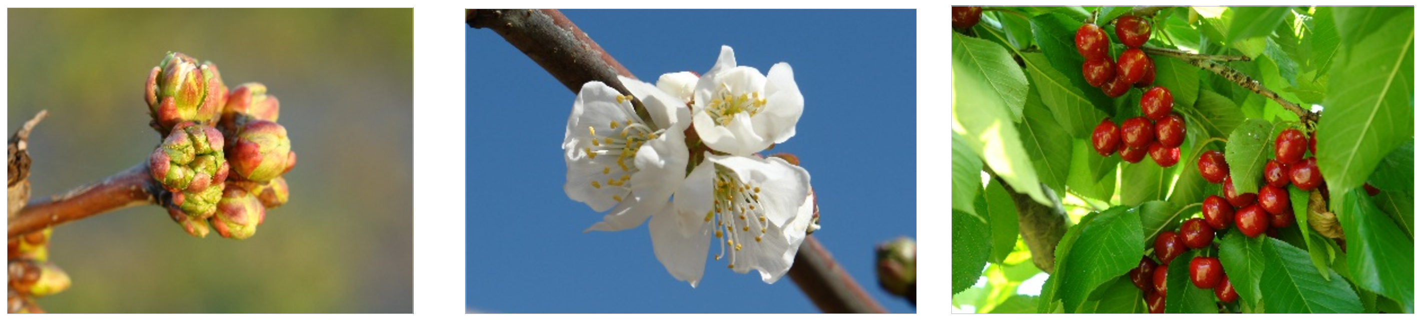{alt=""}
# **04 Climate change and impact projection**
**Drivers of climate change**
- Sun-cyclic variability (evidence: sunspots). Small portion
- Aerosols- suspension of particles (dust, fires, seasalts, manmade), deflects some sunlight from Earth-\> cooling effect. Major driver in industrial areas
- Clouds- can have warming or cooling effect; depends on the type of cloud (varied effects depending on altitude, etc.). Lower= more sunlight reflected. Effect is very complex.
- Ozone- tropospheric ozone (bad ozone, smog); stratospheric ozone (good ozone, blocks UV-B). +GHG -\> warming effect. Destroyed by CFCs (ozone hole in S hemisphere, was fixed when the world took notice and acted-\> *Montreal protocol of 1987*)
- Surface albedo- properties of reflecting surface (land surface); light surfaces-\> more reflection, dark surfaces-\> less reflection
-deforestation- raises albedo
-drying-raises albedo
- feedback loop-accelerates whatever is in place
-less ice/snow-\>lower albedo-\> less heat reflection-\>warming
- GHGs (CO2, CH4, N2O)- atmospheric gases that absorb long-wave radiation (traps heat)-\> warming effect
-N2O, CH4\~ agriculture
- Long term drivers- trends in solar activity (star life cycle); ocean currents/continents; plants/animals (hypothetical)- imbalance of CO2 (heating due to higher CO2)-\> flipping between "Snowball Earth" and "Greenhouse Earth"; volcanic and meteorite activity; Milankovic cycles (variation in tilt, eccentricity, precession of Earth's orbit)
these factors are quantifiable: attribution studies
models have been crafted, compared to observed, and the recent increase(since industrialization) in global temperature can be explained by GHGE from human activities (burning of fossil fuels)
trends of CO2 emissions is still going up (new climatic territories)
degree of CO2 concentrations never seen by mankind, at high rates
**Recent warming**
Starting around 1980s, there is dramatic rise in global temperatures. Globally warmest years are very recent.
-\> Siberia (2020) \>8C warmer (possibility of +feedback=acceleration of warming effect)
Maunder minimum-\> minimal sunspots, low solar radiation
Industrialization- GHGEs
Global surface temperatures started with warming, then a long period of cooling.
+1.5C is optimistic expectation (global temperature increase), but still requires adaptation-\> +5C would cause major global changes unseen before by mankind
Rainfall is harder to predict than temperatures (no clear trends)
Moisture deficit in EU
Places with airports= good data (weather stations)
**Future Scenarios**
No way of validating which scenario is correct
- GCM (Global Circulation Models)- computational effort (major drivers, feedbacks considered)
Climate drivers
Scenarios (fossil-intensive, low emissions, high emissions, intermediate)
- RCPs (Representative Concentration Pathways)
2.6, 4.5, 6.0, 8.5- additional radiative forcing; higher number, more heating (higher emissions)
Downscaling (Dynamical downscaling, Statistical downscaling)- needed to increase resolution (more detail)
GCM\>RCM\>Impact Model
Statistical downscaling- higher resolution
-\> use high resolution temp map, calculate diff between temperature map and average of pixel of RCM, delta change procedure (calculate bias), correct output using bias
in chillR, weather generator is implemented to reduce timestep of climate scenarios (temporal downscaling)
- Climate change projection process
RCPs\> GCM \> downscaling (RCM) \> statistical downscaling\>Temperature, Precipitation, CO2 projections \> Impact projection (e.g. what will happen to a certain species; biological response)
many ways to do process (no way to tell which is best), do all of the combinations and see what the models say
gap: in context of agriculture, models are created by data scientists who are not agricultural experts, there are gaps
- Risk assessment (agricultural context)- additional step needed to project impacts in agriculture
**Future temperatures**
RCP 8.5: rise of 2 to 11C in global temperatures
Tipping point- point of sudden transition to new state (poorly considered in impact projections)
-\> meltwater from Greenland dilutes salt concentration, less driver for global ocean currents (cold, salty water is heaviest); further slowing= transition of global climate to new state
-Greenland, arctic iceloss-\> weakened albedo
-Permafrost thawing-\> CO2 and methane release (more warming)
full of uncertainties
emissions can be translated to temperature increase
Paris Agreement: 1.5C increase only
-\> 2060, CO2 neutral atleast
**Impact Projection**
system response
- Statistical models- climate parameters x impact measure; used to explain past trends and project future impacts
-\> species distribution modeling- climate parameters x presence/absence of species
ensemble modelling- using \>1 approach, check overlaps
e.g. BiodiversityR package
limitations- things change, statistical relationships may not remain true; missing important factors; assumption: species distribution is in equilibrium with climate (x agricultural setups); must state uncertainties explicitly
- Process-based models- computation, data, simulation to get quantitative projection of performance (e.g. crop models, phenology models, etc.); complex since need to include all relevant system components
projection of crop yields (limitations: does not consider real life threats-\> diseases, weeds, etc.)
limitations- processes not completely understood; complex systems not modeled realistically; unclear uncertainties
complexity vs precision (more parameters, more errors)- aim for intermediate complexity to minimize errors "sweet spot"
express uncertainties and error estimates (always)
yield projections are complex, more uncertainties
*before doing such projections, make sure you have a way to quantify the uncertainties!*
- Climate analogue models- comparing similar existing climates with projected climates; adaptation options
limitations: (analog vs target) other factors may be too similar-\> cannot learn new things; other factors may be too different (e.g. cultural management, etc.)-\>too complex to model, huge uncertainties
Common limitations: climate data are scarce or poor quality; non-climatic factors also change through time, and difficult to project; CO2 can only be included in process-based models
Projecting climate-change impacts in complex agricultural systems:
need to understand what is happening: weather, climate, and crops + all other relevant factors affecting system performance; consider and communicate uncertainties
Exercise:
1. Main drivers of climate change (decade to century scale), explain mechanism through which the currently most important driver affects our climate.
*at century scale:* Sun (radiation), Aerosols (liquid,solid, mixed suspensions), Clouds (cooling and warming effect), Ozone (destroyed by CFCs, Montreal protocol of 1987), Surface albedo (reflects radiation) , GHGs, long term drivers (solar activity trends, ocean currents, plants vs animals, volcanic and meteorite activity, milankovic cycles)
*mechanism through which most important driver affects climate:* rising concentration of GHGs-\> this is due to activities of mankind. CO2, CH4, and SO2 are released into the atmosphere. These stay in the atmosphere for very long periods and absorb long-wave radiation, which causes heating up of the Earth; thus causing "greenhouse effect".
2. Explain briefly what is special about temperature dynamics of the recent decades, and why we have good reasons to be concerned.
Industrial revolution led to sharp rise in global temperatures (land, ocean surface temperatures) never seen before by mankind. A world that is quickly becoming \>1.5C hotter than now would require tremendous adaption effort from future generations. Since we have not seen it before, the fear of uncertainty and looming feeling of doom is a great motivation to take GHGE reduction seriously; or else we might say 'hi' to dinosaurs sooner than we think.
3. What does the abbreviation 'RCP' stand for, how are RCPs defined, and what is their role in projecting future climates?
RCP: Representative Concentration Pathways. Each RCP is defined by additional radiative forcing; the higher the number, the higher the emissions and global heating. Currently, the commonly used ones are: RCP 2.6, 4.5, 6.0, 8.5, order is from the most conservative to the most emission-intensive estimate.
Impact projection starts at identifying RCPs -\> inputs for climate change impact models. Process is as follows:
RCPs\> GCM \> downscaling (RCM) \> statistical downscaling\>Temperature, Precipitation, CO2 projections \> Impact projection
4. Briefly describe the 4 climate impact projection methods described in the fourth video.
a\. Statistical models- climate parameters x impact measure; used to explain past trends and project future impacts
b\. Species distribution modelling- climate parameters x presence/absence of species.
c\. Process-based models- use of mathematical equations to quantify system components and processes involved, and to project climate impact to the system. Complex since all relevant factors must be included (non-climatic); resource-intensive and requires processing of huge data
d\. Climate analogue models- involves the use of a similar and existing location where the climate projection can be compared to. Target x analog locations
# **05** Winter chill projections
Chilling hours- hours of low temperature required to break fruit dormancy during winter. Various models have different definitions (Kaufmann, 2019):
- Weinberger (1950): 1 CH=number of hours 0-\>7.2C
- Utah model (1974): 1 CU= 1.4-\>12.4C
- Dynamic model (1987): CP= -2-\> 12C; optimal chilling 6-\>8C
Apples- 500 to 1000 CH
1 CP= 10 CH
Exercise:
1. Sketch out three data access and processing challenges that had to be overcome in order to produce chill projections with state-of-the-art methodology.
-limitation of equipment/available infrastructure in processing huge chunk of data
-incomplete or lack of high resolution climate datasets for some places; would need to make estimates (ground for errors) with respect to nearby places with available data
-form in which data is available in (especially for really large data); data in raster form adds additional steps before they can be rendered usable
2. Outline, in your understanding, the basic steps that are necessary to make such projections.
understand context and systems in location chosen (research + literature review)-\> form your research question -\> choose the appropriate chill model and climate projection ensembles to use -\> obtain data needed for the chosen model-\> interpolate/make estimates if there gaps -\> process data using the model -\> compare projections with existing projections/historic observations -\> conclusion + expression of uncertainties and errors
# **06** Manual chill analysis
CH computation requirement: hourly data;
`read.table` or `read.csv` functions;
.xls or .xlsx `winters_hours_gaps` dataset `kable` format for improved aesthetic;
`<-` assigning new values to R objects comparison commands (`<`, `<=`, `==`, `=>` and `>`);
`c()` command creates strings of numbers "vectors";
`&` command combines comparisons;
`FALSE` and `TRUE` \~ `0` and `1` `which` command to identify items in dataset of interest
Creating functions:
`OurFunctionName <- function(argument1, argument2, ...) {ourCode}`
Exercises:
1. Write a basic function that calculates warm hours (\>25°C)
```{r, eval=FALSE}
Year<-c(2000:2010)
Temps<-c(20:30)
randomdataset<-data.frame(Year, Temps)
##function creation, assigning of threshold to variable
WH<- function(randomdataset)
{
threshold_warm<- 25
randomdataset[,"Warm_year"]<- randomdataset$Temps>threshold_warm
return(randomdataset)
}
sampleWH<-WH(randomdataset)
write.csv(sampleWH, "data/sampleWH.csv", row.names = FALSE)
```
```{r, echo=FALSE}
library(kableExtra)
library(chillR)
sampleWH<-read_tab("data/sampleWH.csv")
WH<-read_tab("data/sampleWH.csv")
kable(head(WH)) %>%
kable_styling("striped", position = "left",font_size = 10)
```
2. Apply this function to the Winters_hours_gaps dataset
```{r, eval=FALSE}
library(knitr)
library(pander)
library(kableExtra)
library(chillR)
##function creation applied to Winter_hours_gaps; I made a new column that tells whether the temperatures are greater than the set threshold value: 25C
hourtemps<- Winters_hours_gaps[,c("Year", "Month", "Day", "Hour", "Temp")]
WH<- function(hourtemps)
{
threshold_warm<- 25
hourtemps[,"Warm_Hour"]<- hourtemps$Temp>threshold_warm
return(hourtemps)
}
write.csv(WH(hourtemps),"data/WH.csv", row.names = FALSE)
```
```{r, echo=FALSE}
library(chillR)
library(kableExtra)
WH<-read_tab("data/WH.csv")
kable(head(WH)) %>%
kable_styling("striped", position = "left",font_size = 10)
```
3. Extend this function, so that it can take start and end dates as inputs and sums up warm hours between these dates
```{r, eval=FALSE}
library(chillR)
##function creation applied to Winter_hours_gaps; I made a new column that tells whether the temperatures are greater than the set threshold value: 25C
hourtemps<- Winters_hours_gaps[,c("Year", "Month", "Day", "Hour", "Temp")]
WH<- function(hourtemps)
{
threshold_warm<- 25
hourtemps[,"Warm_Hour"]<- hourtemps$Temp>threshold_warm
return(hourtemps)
}
WH(hourtemps)[13:20,]
##sum of warm hours of start date and end year in YEARMODA
sum_WH<-function(hourtemps, Start_YEARMODA, End_YEARMODA)
{
Start_Year<-trunc(Start_YEARMODA/10000)
Start_Month<- trunc((Start_YEARMODA-Start_Year*10000)/100)
Start_Day<- Start_YEARMODA-Start_Year*10000-Start_Month*100
Start_Hour<-12
End_Year<-trunc(End_YEARMODA/10000)
End_Month<- trunc((End_YEARMODA-End_Year*10000)/100)
End_Day<- End_YEARMODA-End_Year*10000-End_Month*100
End_Hour<-12
Start_Date<-which(hourtemps$Year==Start_Year & hourtemps$Month==Start_Month & hourtemps$Day==Start_Day & hourtemps$Hour==Start_Hour)
End_Date<-which(hourtemps$Year==End_Year & hourtemps$Month==End_Month & hourtemps$Day==End_Day & hourtemps$Hour==End_Hour)
Warm_hours<- WH(hourtemps)
return(sum(Warm_hours$Warm_Hour[Start_Date:End_Date]))
}
```
```{r, eval=FALSE}
##sample content for checking. # of warm hours in set time interval by manual counting= using sum_WH function), so I confirmed there's no error anywhere
sum_WH(hourtemps,20080517,20080518)
WH(hourtemps)[1803:1827,]
```
```{r, echo=FALSE}
library(kableExtra)
WH_sample<-read_tab("data/WH.csv")
kable(WH_sample[1803:1827,]) %>%
kable_styling("striped", position = "left",font_size = 10)
```
```{r, eval=FALSE}
##[1] 15
```
# **07** Chill models
CH model- not credible
Utah Model- more credible (different weights for different temperatures
Dynamic Model- complex, needs heavy maths.
`Chilling_Hours()` function determines if each hour are within 0 to 7.2C ;
`step_model()` function- allows user to define model (set thresholds and weights);
`summ==TRUE` cumulative sum;
`data.frame`- input, contains weights for temperature ranges; `custom()` function implements chill model based on set;
`data.frame` input `make_JDay()` function adds Julian dates;
`chilling()` function implements CH, Utah, and Dynamic models, and computes GDH (Growing Degree Days);
`tempResponse` function lets user pick what model they want in `chilling()` function
Exercise:
1. Run the `chilling()` function on the `Winters_hours_gap` dataset
```{r, eval=FALSE}
library(chillR)
chill_sample<-chilling(make_JDay(Winters_hours_gaps),Start_JDay = 90, End_JDay = 100)
write.csv(chill_sample, "data/chill_sample.csv", row.names = FALSE)
```
```{r,echo=FALSE}
chill_sample<-read_tab("data/chill_sample.csv")
kable(head(chill_sample)) %>%
kable_styling("striped", position = "left",font_size = 10)
```
2. Create your own temperature-weighting chill model using the `step_model()` function
I looked at Milech et. al (2018) to see other existing models I have not seen yet so far in this module, and saw a nice table from [their study](https://www.researchgate.net/publication/331103354_MODELS_TO_ESTIMATE_CHILLING_ACCUMULATION_UNDER_SUBTROPICAL_CLIMATIC_CONDITIONS_IN_BRAZIL) summarizing models and the ranges. I picked **Low Chill Model** to be my guinea pig for this exercise portion; I did not use its equations, **only the temperature ranges and weights**.
```{r, eval=FALSE}
##implementing the ranges from Low Chill Model
df<-data.frame(
lower= c(-1000, 1.8, 7.9, 13.9, 16.9, 19.4, 20.4),
upper=c(1.8, 7.9,13.9,16.9, 19.4, 20.4, 1000),
weight=c(0, 0.5, 1, 0.5, 0, -0.5, -1)
)
custom<- function(x) step_model(x, df)
##sample values for first 100 rows from the Winters_hours_gaps dataset)
custom(Winters_hours_gaps$Temp)[1:100]
write.csv(custom(Winters_hours_gaps$Temp), "data/custom.csv", row.names = FALSE)
```
```{r, echo=FALSE}
custom<-read_tab("data/custom.csv")
kable(head(custom)) %>%
kable_styling("striped", position = "left",font_size = 10)
```
3. Run this model on the `Winters_hours_gaps` dataset using the `tempResponse()` function.
```{r, eval=FALSE}
df<-data.frame(
lower= c(-1000, 1.8, 7.9, 13.9, 16.9, 19.4, 20.4),
upper=c(1.8, 7.9,13.9,16.9, 19.4, 20.4, 1000),
weight=c(0,0.5, 1, 0.5, 0, -0.5, -1)
)
custom<- function(x) step_model(x, df)
output<-tempResponse(make_JDay(Winters_hours_gaps), Start_JDay = 90, End_JDay = 100, models=list(custom=custom))
write.csv(output, "data/output.csv", row.names = FALSE)
```
```{r, echo=FALSE}
output<-read_tab("data/output.csv")
kable(head(output)) %>%
kable_styling("striped", position = "left",font_size = 10)
```
# **08** Making hourly temperatures
`daylength` function- generates daily temperature curves from the latitude input;
`ggplot2` package- for plotting;
JDay= Julian Date (1 to 365 or 366 in leap years);
`melt` command of the `reshape2` package- separates/melts dataframe, stacked; `stack_hourly_temps()` function integrates daily dynamics using minimum and maximum temperature data + latitude;
`KA_weather` dataset contains temperature data from Bonn Uni; `Empirical_daily_temperature_curve()` function determines typical temperatures at locations; `make_all_day_table` function fills gaps in daily and hourly temperature records
Exercise:
1. Choose a location of interest, find out its latitude and produce plots of daily sunrise, sunset and daylength.
I have always been fascinated with Nordic mythology-- Vikings. Sometimes I ask myself: why don't we just consult the three Norns who spin the webs of fate: *Urd* (Past), *Verdandi* (Present), and *Skuld* (future) instead of modelling climate scenarios? Would be a *cooler* way to predicting the *heating* of Earth! Below is a fun image of the three Norns I got from a [Norse Mythology website](https://norse-mythology.org/wp-content/uploads/2012/11/Norns.jpg).

My Nordic tale-loving soul convinced me to look at interesting locations in Norway, Sweden, and Denmark. I narrowed down my search by looking at the ranking of countries with the most number of weather stations, and voila! got my answer: **Sweden**. The plot below shows the number of weather stations across the globe from [Jaffre (2019).](https://www.researchgate.net/publication/326343778_GHCN-Daily_a_treasure_trove_of_climate_data_awaiting_discovery)

An [interesting project](https://www.fruit-processing.com/2020/02/large-scale-apple-growing-in-northern-sweden/) implemented in Northern Sweden by Brännland Cider (a Swedish company making ice cider from apples) caught my attention. European innovation partnership for productivity and sustainability within agriculture (EIP-agri) of the Swedish Board of Agriculture granted them around 935,000 euro for this. The aim is to pilot climate-resilient agriculture in the Northern EU by trying to grow apples commercially in the harsh northern climate. The three counties involved are: Norrbotten, Västerbotten and Västernorrland; and I picked **Västerbotten** ([64.34° N, 18.31° E](https://latitude.to/articles-by-country/se/sweden/25937/vasterbotten-county)) because it had many airports close to it-- nearest was 12 km away. It would be very interesting to know what the field trials would look years in the future temperature-wise. *Would they be able to make ice cider decades from now in that area?*
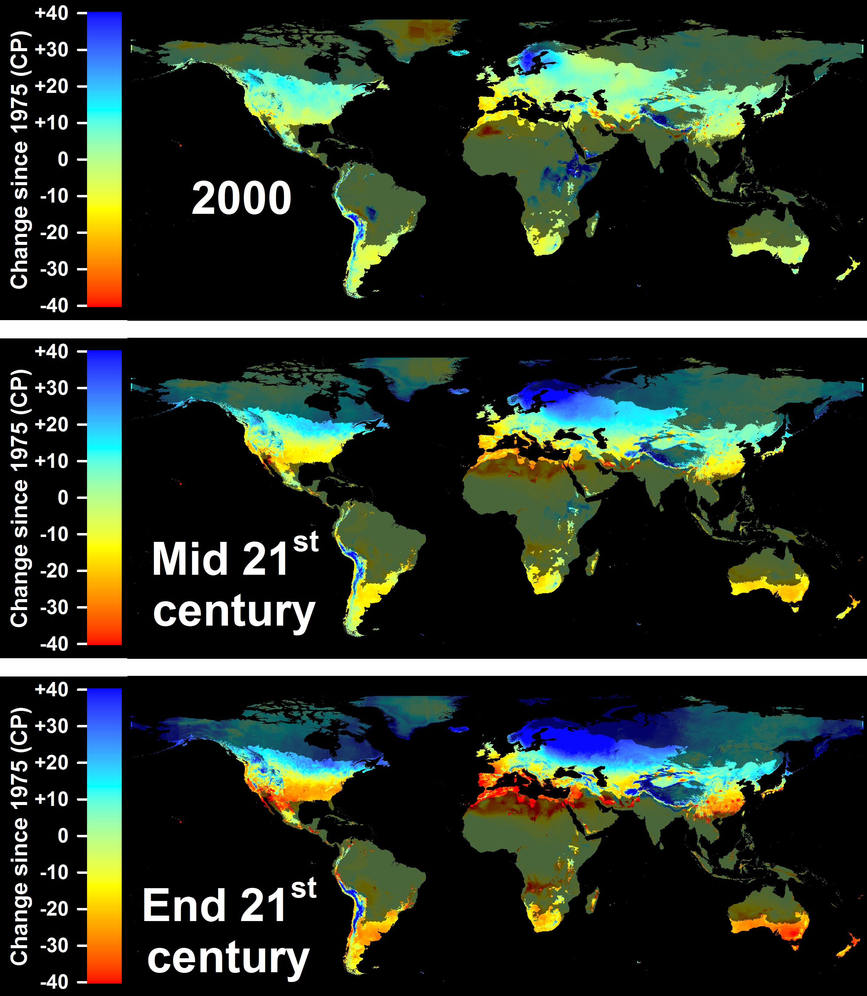
I kept in mind that the location will be used repeatedly for the next topics so I chose quite strategically. Though my expectation is that they will be able to continue to grow apples because that region will not get warmer as per [previous projections](http://inresgb-lehre.iaas.uni-bonn.de/chillR_book/winter-chill-projections.html) by Luedeling et al. (2011):
Now, for the exercise,
```{r, eval=FALSE}
require(chillR)
require(ggplot2)
require(reshape2)
Days<-daylength(latitude=64.34, JDay=1:365)
Days_df<-data.frame(JDay=1:365, Sunrise=Days$Sunrise, Sunset=Days$Sunset, Daylength=Days$Daylength)
Days_df<-melt(Days_df, id=c("JDay"))
ggplot(Days_df, aes(JDay, value))+ geom_line(lwd=1.5) + facet_grid(cols=vars(variable))+ylab("Time of Day/Daylength (Hours)")+ theme_bw(base_size=20)
```

2. Produce an hourly dataset, based on idealized daily curves, for the `KA_weather` dataset (included in `chillR`)
```{r, eval=FALSE}
require(chillR)
KA_weather_stacked<-stack_hourly_temps(KA_weather, latitude=64.34)
write.csv(KA_weather_stacked, "data/KA_weather_stacked.csv", row.names = FALSE)
```
```{r, echo=FALSE}
require(kableExtra)
KA_weather_stacked<-read_tab("data/KA_weather_stacked.csv")
kable(head(KA_weather_stacked)) %>%
kable_styling("striped", position = "left",font_size = 10)
```
3. Produce empirical temperature curve parameters for the `Winters_hours_gaps` dataset, and use them to predict hourly values from daily temperatures (this is very similar to the example above, but please make sure you understand what's going on)
```{r, eval=FALSE}
library(chillR)
library(ggplot2)
##determining empirical daily temperatures from hourly data using Winters_hours_gaps dataset
coeffs<-Empirical_daily_temperature_curve(Winters_hours_gaps)
Winters_daily<-make_all_day_table(Winters_hours_gaps, input_timestep="hour")
Winters_hours<-Empirical_hourly_temperatures(Winters_daily,coeffs)
?Winters_hours_gaps
##input latitude of Winters, California (38.5 N) where Winters_hours_gaps dataset was recorded in
require(reshape2)
Winters_hours<-Winters_hours[,c("Year","Month","Day","Hour","Temp")]
colnames(Winters_hours)[ncol(Winters_hours)]<-"Temp_empirical"
Winters_ideal<-stack_hourly_temps(Winters_daily, latitude=38.5)$hourtemps
Winters_ideal<-Winters_ideal[,c("Year","Month","Day","Hour","Temp")]
colnames(Winters_ideal)[ncol(Winters_ideal)]<-"Temp_ideal"
##Triangular dataset
Winters_triangle<-Winters_daily
Winters_triangle[,"Hour"]<-0
Winters_triangle$Hour[nrow(Winters_triangle)]<-23
Winters_triangle[,"Temp"]<-0
Winters_triangle<-make_all_day_table(Winters_triangle,timestep="hour")
colnames(Winters_triangle)[ncol(Winters_triangle)]<-"Temp_triangular"
for(i in 2:nrow(Winters_triangle))
{if(is.na(Winters_triangle$Tmin[i])) Winters_triangle$Tmin[i]<-Winters_triangle$Tmin[i-1]
if(is.na(Winters_triangle$Tmax[i])) Winters_triangle$Tmax[i]<-Winters_triangle$Tmax[i-1]
}
Winters_triangle$Temp_triangular<-NA
Winters_triangle$Temp_triangular[which(Winters_triangle$Hour==6)]<-
Winters_triangle$Tmin[which(Winters_triangle$Hour==6)]
Winters_triangle$Temp_triangular[which(Winters_triangle$Hour==18)]<-
Winters_triangle$Tmax[which(Winters_triangle$Hour==18)]
Winters_triangle$Temp_triangular<-
interpolate_gaps(Winters_triangle$Temp_triangular)$interp
Winters_triangle<-Winters_triangle[,c("Year","Month","Day","Hour","Temp_triangular")]
##merging the dataframes
Winters_temps<-merge(Winters_hours_gaps,Winters_hours, by=c("Year","Month","Day","Hour"))
Winters_temps<-merge(Winters_temps,Winters_triangle, by=c("Year","Month","Day","Hour"))
Winters_temps<-merge(Winters_temps,Winters_ideal, by=c("Year","Month","Day","Hour"))
##conversion of dates, reorganizing dataframes, plotting
Winters_temps[,"DATE"]<-ISOdate(Winters_temps$Year,Winters_temps$Month, Winters_temps$Day, Winters_temps$Hour)
Winters_temps_to_plot<-Winters_temps[,c("DATE","Temp","Temp_empirical","Temp_triangular","Temp_ideal")]
Winters_temps_to_plot<-Winters_temps_to_plot[100:200,]
Winters_temps_to_plot<-melt(Winters_temps_to_plot, id=c("DATE"))
colnames(Winters_temps_to_plot)<-c("DATE","Method","Temperature")
ggplot(data=Winters_temps_to_plot, aes(DATE,Temperature, colour=Method)) +
geom_line(lwd=1.3) + ylab("Temperature (°C)") + xlab("Date")
```

# **09** Getting temperature data
GSOD- Global Summary of Day database
ChillR only has access to GSOD and California database
`handle_gsod()` function for data retrieval from GSOD;
`Overlap_years` column shows \# years available;
`Perc_interval_covered` column shows % that target (start-end date input) was covered
Exercise:
1. Choose a location of interest and find the 25 closest weather stations using the `handle_gsod` function
Will use Västerbotten, Sweden ([64.34° N, 18.31° E](https://latitude.to/articles-by-country/se/sweden/25937/vasterbotten-county)) again.
```{r, eval=FALSE}
library(chillR)
##generation of station list based on target location's coordinates
station_list_Västerbotten<-handle_gsod(action="list_stations",
location=c(18.31,64.34),
time_interval=c(1990,2020))
write.csv(station_list_Västerbotten, "data/station_list_Västerbotten.csv")
```
```{r, echo=FALSE}
library(kableExtra)
station_list_Västerbotten<-read_tab("data/station_list_Västerbotten.csv")
kable(head(station_list_Västerbotten)) %>%
kable_styling("striped", position = "left",font_size = 10)
```
2. Download weather data for the most promising station on the list
From the 25 stations nearest the chosen location, the **fifth (Lycksele, ChillR code 022610-99999)** was the most promising; it covered 100% of the data for 1990 to 2020. Though it was quite far in terms of distance from the target area.
```{r, eval=FALSE}
library(chillR)
##generation of station list based on target location's coordinates
station_list<-handle_gsod(action="list_stations",
location=c(18.31,64.34),
time_interval=c(1990,2020))
##having to enter just the number of station from the list created was a relief, thanks chillR coders!
weather<-handle_gsod(action="download_weather",
location=station_list$chillR_code[5],
time_interval=c(1990,2020))
##check sample data
weather[[1]]$weather[5090:6010,]
#downloading data
write.csv(weather,"data/Västerbotten_weather.csv",row.names=FALSE)
```
```{r, echo=FALSE}
library(kableExtra)
Västerbotten_weather<-read_tab("data/Västerbotten_weather.csv")
kable(head(Västerbotten_weather)) %>%
kable_styling("striped", position = "left",font_size = 10)
```
3. Convert the weather data into `chillR` format
```{r, eval=FALSE}
library(chillR)
##generation of station list based on target location's coordinates
station_list<-handle_gsod(action="list_stations",
location=c(18.31,64.34),time_interval = c(1990,2020))
##having to enter just the number of station from the list created was a relief, thanks chillR coders!
weather<-handle_gsod(action="download_weather",
location=station_list$chillR_code[5],
time_interval=c(1990,2020))
##datacleaning, changing format to chillR
cleaned_weather<-handle_gsod(weather)
##check sample cleaned data, I used a non-boring range
cleaned_weather[[1]]$weather[5090:6010,]
##downloading data for future use
write.csv(cleaned_weather$weather,"data/Västerbotten_chillR_weather.csv",row.names=FALSE)
```
```{r, echo=FALSE}
library(kableExtra)
Västerbotten_weather_clean<-read_tab("data/Västerbotten_chillR_weather.csv")
kable(head(Västerbotten_weather_clean)) %>%
kable_styling("striped", position = "left",font_size = 10)
```
From the looks of the data I got as shown above from Västerbotten taken from GSOD database, it's **not possible** to work with it for the next exercises. I already tried doing first exercise in Chapter 10 and it failed to be read using read.csv function (contains no data, that also happened to Bonn weather example from GSOD I ran). So for the next exercises, I would have to choose another location, possibly in Germany since the **DWD database** seems working well with chillR. To be able to move forward, I will also use DWD database for the filling of gaps exercise.
Another reason is we already know that Nordic regions will remain cold enough anyway as per previous projections. Makes me sad though; but will not cry because I am a tough Viking by heart.
# 10 Getting temperature data
linear interpolation can be done to fill in short gaps (hours to weeks), but longer gaps need better methods to reflect temperature dynamics
`interpolate_gaps()` function carries out simple interpolation; `fix_weather()` function uses linear interpolation between Tmax and Tmin columns and can be used to identify gaps in the dataset
Exercise:
1. Use `chillR` functions to find out how many gaps you have in this dataset (even if you have none, please still follow all further steps)
I will repeat the previous steps done in the last exercise in this portion. New location of choice is the [Swabian Orchard Paradise](https://www.streuobstparadies.de/) (48.4931° N, 9.3998° E) near Stuttgart. I had the chance to visit a Schwabian place before and ate some of their local dishes, courtesy of the tour by my mentor [Martin Gummert](https://www.researchgate.net/profile/Martin-Gummert). The orchard grows cherries, pears, and plums-- and it is said that it has been centuries-old; would be interesting to check if they will survive another century.
A quick view of the place I got from [Schwäbisches Streuobstparadies Website](https://www.streuobstparadies.de/var/streu/storage/images/streu_bw-karte/16427-1-ger-DE/STREU_BW-Karte_front_large.jpg) (n.d.):

Now onto the code:
```{r, eval=FALSE}
library(chillR)
##generation of list, handle DWD dataset
station_list_dwd<-handle_dwd(action="list_stations",
location=c(9.40,48.49),
time_interval=c(19900101,20201231))
##check weather station list
require(kableExtra)
kable(station_list_dwd) %>%
kable_styling("striped", position = "left", font_size = 8)
##the list showed M<fc>nsingen-Apfelstetten (station 654) as the nearest and most number of years available (1946 to 2021), so I am choosing it (#2 in the station list)
##downloading the data from chosen weather station and checking data
weather_dwd<-handle_dwd(action="download_weather",
location=station_list_dwd$Station_ID[2],
time_interval=c(19900101,20201231))
head(weather_dwd$`M<fc>nsingen-Apfelstetten`$weather)
##datacleaning and checking data
cleaned_weather_dwd<-handle_dwd(weather_dwd)
cleaned_weather_dwd$`M<fc>nsingen-Apfelstetten`
##saving data in computer
write.csv(station_list_dwd,"data/station_list_dwd.csv",row.names=FALSE)
write.csv(weather_dwd,"data/MApfelstetten_weather1.csv",row.names=FALSE)
write.csv(cleaned_weather_dwd$`M<fc>nsingen-Apfelstetten`,"data/MApfelstetten_chillR_weather.csv",row.names=FALSE)
##assigning previous data to an object
MApfelstetten<-read.csv("data/MApfelstetten_chillR_weather.csv")
#checking for gaps using fix_weather function
MApfelstetten_QC<-fix_weather(MApfelstetten)$QC
write.csv(MApfelstetten_QC, "data/MApfelstetten_QC.csv", row.names = FALSE)
##saving and downloading the needed columns for next exercises
MApfelstetten_weather<-MApfelstetten[,c("Year","Month", "Day", "Tmax", "Tmin")]
kable(MApfelstetten_weather,) %>%
kable_styling("striped", position = "left", font_size = 10)
write.csv(MApfelstetten_weather, "data/MApfelstetten_weather.csv", row.names = FALSE)
```
```{r, echo=FALSE}
MApfelstetten_QC<-read_tab("data/MApfelstetten_QC.csv")
kable(head(MApfelstetten_QC), caption="Quality control summary produced by *fix_weather()*") %>%
kable_styling("striped", position = "left", font_size = 10)
```
```{r, echo=FALSE}
library(kableExtra)
MApfelstetten_weather<-read_tab("data/MApfelstetten_weather.csv")
kable(head(MApfelstetten_weather)) %>%
kable_styling("striped", position = "left", font_size = 10)
```
Surprise, surprise! according to the results from running the `fix_weather()` function, there is **no gap for the Münsingen-Apfelstetten weather station** (DWD database) for our years of interest.
So now, I will create artificial gaps by deleting some data from the original dataset and work with filling it for the next exercises. The dataset I am using is [here](https://github.com/GraceBarbacias/Tree-Phenology-using-R_files/blob/main/MApfelstetten_chillR_weather_gaps.csv).
```{r, eval=FALSE}
library(chillR)
##assigning previous data to an object
MApfelstetten_gaps<-read.csv("data/MApfelstetten_chillR_weather_gaps.csv")
#checking for gaps using fix_weather function
MApfelstetten_QC_gaps<-fix_weather(MApfelstetten_gaps)$QC
write.csv(MApfelstetten_QC_gaps, "data/MApfelstetten_QC_gaps.csv", row.names = FALSE)
```
```{r, echo=FALSE}
MApfelstetten_QC_gaps<-read_tab("data/MApfelstetten_QC_gaps.csv")
kable(head(MApfelstetten_QC_gaps), caption="Quality control summary produced by *fix_weather()*") %>%
kable_styling("striped", position = "left", font_size = 10)
```
This confirmed the existence of gaps in 1990, 1991, 2004, 2005, 2012, 2018, 2019, and 2020.
2. Create a list of the 25 closest weather stations using the `handle_gsod` function
I will use the location of the Swabian Orchard Paradise (48.4931° N, 9.3998° E) to check weather stations around via the `handle_dwd` function.
```{r,eval=FALSE}
library(chillR)
library(kableExtra)
##generation of list, handle DWD dataset
station_list_dwd<-handle_dwd(action="list_stations",
location=c(9.40,48.49),
time_interval=c(19900101,20201231))
```
```{r, echo=FALSE}
station_list_dwd<-read_tab("data/station_list_dwd.csv")
kable(head(station_list_dwd), caption="Quality control summary produced by *fix_weather()*") %>%
kable_styling("striped", position = "left", font_size = 10)
```
3. Identify suitable weather stations for patching gaps
There are weather stations in the DWD list that are mostly complete *I think*, but for the sake of me trying to create a list (and we can never be sure that they indeed contain complete data with just the range of years shown), I will try to use 3 stations: **1, 3, and 6** from the weather station list.
4. Download weather data for promising stations, convert them to `chillR` format and compile them in a list
```{r, eval=FALSE}
##attempt 3
require(reshape2)
require(kableExtra)
require(ggplot2)
library(chillR)
station_list_dwd<-handle_dwd(action="list_stations",location=c(9.40,48.49),time_interval=c(19900101,20201231))
positions_in_station_list<-c(1,3,6)
patch_weather<-list()
for(i in 1:length(positions_in_station_list))
{patch_weather[[i]]<-handle_dwd(handle_dwd(action="download_weather",
location=station_list_dwd$Station_ID[positions_in_station_list[i]],time_interval=c(19900101,20211231)))[[1]]
names(patch_weather)[i]<-station_list_dwd$Station_name[positions_in_station_list[i]]
}
save_temperature_scenarios(patch_weather,"data/", "patch_weather")
```
5. Use the `patch_daily_temperatures` function to fill gaps
Instead of Chapter 30, this exercise is the last bit I worked on because I had been wracking my head on how to carry this out when the `patch_daily_temps` seemed to only work perfectly fine with 'gsod' datafiles. So many hiccups because I could not also clean the 'gsod' raw files with `handle_gsod` for some reason. It always returns an empty file. That was the reason I had to use 'dwd' datafiles and move the location to Swabian Orchard paradise.
After so many attempts, I was able to figure out that the 'old and deprecated' function `patch_daily_temperatures` would be able to handle 'dwd' datafiles well-- at least in my case. Please remember that the patched data here is just for the sake of doing this exercise. I will be using the complete authentic data from dwd for my location for the next exercises. So, here's the product of my many hours of sweat and tears:
```{r, eval=FALSE}
require(reshape2)
require(kableExtra)
require(ggplot2)
library(chillR)
##recall previous list()
station_list_dwd<-handle_dwd(action="list_stations",location=c(9.40,48.49),time_interval=c(19900101,20201231))
positions_in_station_list<-c(1,3,6)
patch_weather<-list()
for(i in 1:length(positions_in_station_list))
{patch_weather[[i]]<-handle_dwd(handle_dwd(action="download_weather",
location=station_list_dwd$Station_ID[positions_in_station_list[i]],time_interval=c(19900101,20211231)))[[1]]
names(patch_weather)[i]<-station_list_dwd$Station_name[positions_in_station_list[i]]
}
##assign the dataset with gaps to object
MApfelstetten<-read_tab("data/MApfelstetten_chillR_weather_gaps.csv")
#first patching, I used the old function 'patch_daily_temperatures'
patched<-patch_daily_temperatures(weather = MApfelstetten,
patch_weather = patch_weather)
##to summarize statistics:
# > patched$statistics
#$`Lenningen-Schopfloch`
# mean_bias stdev_bias filled gaps_remain
#Tmin -1.709 2.032 80 1027
#Tmax -0.085 1.283 80 1027
#$`Reutlingen-Betzingen`
# mean_bias stdev_bias filled gaps_remain
#Tmin -2.062 1.664 0 1027
#Tmax -2.999 1.501 0 1027